REVIEW 3 major objections 5 minor 25 references
Learning and Testing Inverse Statistical Problems For Interacting Systems Undergoing Phase Transition
T0 review · 3 major / 5 minor · reviewed 2026-08-06 · deepseek-v4-flash
Pith's one-line read Pseudo-likelihood inference beats mean-field at every temperature
desk verdict A careful, genuinely useful tutorial on inverse statistical mechanics with real code; the headline comparative claim needs error bars, but the paper deserves peer review. read the letter →
The pith
A machine-rendered reading of the paper's core claim, the machinery that carries it, and where it could break.
The reading
What carries the argument
The load-bearing object is the single-site pseudo-likelihood, which replaces the full Boltzmann-Gibbs conditional average over the other $N-1$ spins with an empirical average over the $M$ measured configurations, turning inference into a logistic-regression problem with convex structure per row. The update rules for couplings and fields are steepest-descent equations whose fixed points match empirical magnetizations and correlations; in the Ising case the conditional probability is $P(s_i|\{s_{\setminus i}\}) = (1 + e^{-z_i})^{-1}$, so maximizing the pseudo-likelihood is a sigmoid/logistic regression. The mean-field comparator is the inverse of the empirical covariance matrix, $\beta J^{\rm MF}_{ij} = -(\Gamma^{-1})_{ij}$. The two are judged through the normalized reconstruction error $\gamma_J$ and through rank plots of the sorted inferred couplings.
What would settle it
Generate a controlled dataset for a spin glass on a random graph using a deliberately short, poorly equilibrated Monte Carlo run (e.g., far fewer Monte Carlo sweeps than the autocorrelation time) and check whether the pseudo-likelihood reconstruction error rises sharply relative to the equilibrium-sampling baseline, or, conversely, find any temperature in the paper's own models where the mean-field reconstruction error falls strictly below the pseudo-likelihood one — either result would contradict the claimed uniform superiority.
Extended reading notes
Core claim
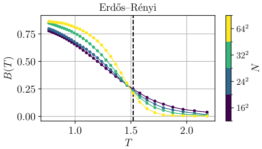
On its own terms, the paper establishes that the max-pseudo-likelihood approach of Sec. III B performs equally or better than the mean-field approach at every temperature. This is shown through the reconstruction error $\gamma_J$ computed over temperature for the Ising model (ordered and bond-disordered, on a square lattice and on Erdős–Rényi graphs), for the $q=4$ Potts clock model (on a cubic lattice and on random graphs), and for the Blume-Capel model (on a square lattice and on random graphs, across both second-order and first-order transition regions). The finding holds across data of 15,000–20,000 Monte Carlo configurations; introducing lasso regularization further lowers the error in the ordered, sparse-coupling cases. The paper also derives the pseudo-likelihood inference as a row-by-row logistic regression and identifies the sampling assumption — that the measured configurations represent the full Boltzmann-Gibbs ensemble — as the premise on which the method is built.
Load-bearing premise
The paper's results stand on the assumption that the $M$ measured Monte Carlo configurations are a statistically representative sample of the full Boltzmann-Gibbs equilibrium ensemble; if the sampling misses entire regions of configuration space — as in glassy low-temperature or first-order-transition regimes — the inferred couplings are biased.
Editorial extensions
If this is right
- Near a phase transition, pseudo-likelihood remains a reliable coupling-reconstruction routine, so practitioners can use it without first knowing whether their data come from the ordered or disordered side.
- When the true interaction network is sparse and ferromagnetic, lasso-regularized pseudo-likelihood is the best of the tested options, producing sharper sorted-coupling plots.
- The rank-plot diagnostic gives a graphical way to check inference quality as a function of dataset size, without needing a known ground truth in application settings.
- Since the method needs only raw configurations and no partition function, it scales to systems where exact maximum likelihood is infeasible.
- The accompanying repository lets a user reproduce the comparisons and apply the pipelines to new models.
Reading between the lines
- The empirical claim is established only on the specific suite of models, temperatures, and dataset sizes used; whether the 'equally or better at every temperature' ordering survives for other topologies (e.g., scale-free graphs), other spin alphabets, or data with measurement noise is a natural testable extension.
- A practical diagnostic suggested by the paper's own caveat: compute an equilibration indicator such as autocorrelation time or the Binder parameter of the input configurations and flag low-confidence inferences where sampling is poor.
- The same pseudo-likelihood machinery, with an appropriate conditional distribution, could be carried over to inverse problems with non-Boltzmann or non-equilibrium data, but the equivalence to logistic regression would no longer guarantee convexity.
Signed reviews
Editorial analysis
A structured set of objections, weighed in public.
Referee Report
Summary. The paper develops and compares three inverse-problem methods—maximum likelihood, maximum pseudo-likelihood (with and without lasso regularization), and naive mean-field—for reconstructing couplings of Ising, q=4 Potts-clock, and Blume-Capel models defined on lattices and Erdős–Rényi graphs. Analytic derivations in Sec. III are followed by numerical estimates of reconstruction error γ_J and rank plots from synthetic equilibrium Monte Carlo data in Sec. IV, with a companion GitHub repository. The central comparative claim is that pseudo-likelihood performs equally or better than mean-field at every temperature.
Significance. The manuscript is a useful didactic synthesis that brings together standard inference techniques and applies them across ferromagnetic, spin-glass, first-order, and tricritical settings. Its strengths include a careful presentation of the pseudo-likelihood derivation, explicit formulas for the Potts and Blume-Capel generalizations, and a public repository that should allow reproduction. The comparative claim, however, is currently supported only by single-realization error curves without uncertainty quantification, so the quantitative benchmark is not yet at the level needed for the stated 'every temperature' conclusion. If the comparison is confirmed with proper statistics, the paper would be a valuable reference for practitioners.
major comments (3)
- [Sec. IV A, Eq. (85), Figs. 5-8] The statement in Sec. IV A 1 that 'the Max-Pseudo-Likelihood approach of Sec. III B performs equally or better than the Mean Field one at every temperature' is not supported by the evidence as presented. The γ_J(T) curves in Figs. 5-8 appear to be single realizations with no error bars, no averaging over independent datasets or initial conditions, and no disorder averaging for the disordered models; the caption of Fig. 6 states that the same graph is used for all data points. With M = 20000 configurations (or 15000 Wolff steps), γ_J is a random quantity whose run-to-run fluctuations, especially near criticality, could be comparable to the apparent gap between the pseudo-likelihood and mean-field curves. Please provide error bars from bootstrapping over configurations or from repeated independent simulations, and state explicitly how many disorder realizations are used, before drawing a conclusion that is uniform in temperature.
- [Sec. III B 4 and Sec. IV A, Figs. 5-7] The lasso results are advertised as further improvements ('Lasso further decreases the error...' in Sec. IV A 1 and analogous statements for Potts and Blume-Capel), but the regularization strength is set ad hoc: λ = 1, 0.01, and 10^-4 for the Ising, Potts, and Blume-Capel cases, respectively. The paper itself notes in Sec. III B 4 that systematic methods such as cross-validation exist. Since λ controls the bias-variance trade-off, the reported lasso improvement may be an artifact of the chosen λ rather than a robust property of the method. At minimum, include a λ-sensitivity analysis or a cross-validated choice for one representative model, and temper the claims about lasso accordingly.
- [Appendix C, Eqs. (C1)-(C2)] The critical temperatures for Erdős–Rényi graphs are computed with BP equations derived for random regular graphs, with the text asserting that 'when a second order transition happens both RR and ER have the same critical temperature.' This is not generally correct as stated. For a ferromagnetic Ising model on an RR graph of degree c, the linear stability of the paramagnetic fixed point in Eqs. (C5)-(C6) gives (c-1) tanh(βJ) = 1, whereas for an ER graph of mean degree c the condition is c tanh(βJ) = 1, Eq. (7). For c = 4 these give different temperatures (approximately 2.885 and 3.912). The paper either needs to clarify that d denotes the mean residual degree of the ER graph (so that d = c, not c-1) or correct the RR/ER equivalence claim; as written, the ER critical lines in Table I, Figs. 2 and 16, and the dashed lines in Figs. 5-8 are not derived consistently.
minor comments (5)
- [Sec. II C] The text 'we take M = 2c/N = 2N' appears to be a typo; with average connectivity c = 4 and N spins, the correct relation is M = cN/2 = 2N.
- [Sec. III B 4] The ℓ1 regularizer for the fields is written as λ_h h_i, but a sparsity-promoting penalty should use |h_i|; please correct the expression, or explain the intended signed penalty.
- [Sec. II A 2] There is a typo in 'phaenomenologu ` ıy' (should be 'phenomenology'), and several other spelling and grammar errors (e.g., 'refereed to' in Sec. III B 4) should be corrected.
- [Appendix B] In the caption of Fig. 18, 'µc ∈ (1.960, 1970)' should read 'µc ∈ (1.960, 1.970)'.
- [Sec. IV B, Figs. 9-12] The rank plots would be easier to interpret if the number of disorder realizations and the temperature at which data are sampled were stated in every caption; currently only some captions give T and β.
Circularity Check
No significant circularity: the inference derivations are self-contained and the comparative numerical claim is an empirical benchmark observation, not a fitted prediction.
full rationale
The paper's derivation chain is self-contained. The maximum-likelihood, pseudo-likelihood, and mean-field formulas in Secs. III A-III C are derived from the Boltzmann-Gibbs measure using standard identities; Eqs. (27)-(34) are exact reformulations before the M-configuration approximation in Eq. (34), and the mean-field inversion beta*J_ij = -(Gamma^{-1})_ij follows from the variational free-energy calculation in Eqs. (71)-(83). No fitted parameter is later relabeled as a prediction: the reconstruction error gamma_J in Eq. (85) compares inferred couplings against the known couplings used to generate synthetic data, and the lasso strengths are reported as heuristic settings, not as inferred outputs. Self-citations (e.g., Refs. 23-28, 51, 53, 57, 63) appear as application examples, pedagogical references, or physical-context citations and are not load-bearing for the central derivation or for the numerical comparison. The paper explicitly flags its main assumption in Sec. III B: 'The sampling is, thus, assumed to be statistically representative of the whole set of configurations. This is the fundamental hypothesis over which the max Pseudo-Likelihood approach is built.' This is a stated modeling assumption, not a circular reduction. The claim that pseudo-likelihood performs 'equally or better' than mean-field is an empirical observation on synthetic benchmarks; the lack of error bars in Figs. 5-8 is a statistical-evidence concern, not a circularity. No self-definitional, fitted-input-as-prediction, self-citation-load-bearing, or author-imported-uniqueness step was found.
Assumptions & free parameters
free parameters (3)
- lasso regularization parameter (Ising) =
1 (Fig. 5)
- lasso regularization parameter (Potts) =
0.01 (Fig. 6)
- lasso regularization parameter (Blume-Capel) =
1e-4 (Fig. 7)
assumptions (5)
- domain assumption Data are generated from a Boltzmann-Gibbs equilibrium distribution (Eq. 12).
- domain assumption Monte Carlo samples are thermalized and effectively independent.
- domain assumption The M sampled configurations are statistically representative of the full 2^{N-1} ensemble (Eq. 34).
- domain assumption Mean-field factorization of the joint probability distribution (Eq. 55 or 71).
- domain assumption Belief Propagation on random regular graphs gives the critical temperature for Erdős-Rényi graphs.
Cite this review
Pith. "Pith review of Learning and Testing Inverse Statistical Problems For Interacting Systems Undergoing Phase Transition." pith.science (2026). https://pith.science/paper/T6FHCHTG
@misc{pith2026250702574,
  author       = {Pith},
  title        = {Pith review of: Learning and Testing Inverse Statistical Problems For Interacting Systems Undergoing Phase Transition},
  year         = {2026},
  howpublished = {\url{https://pith.science/paper/T6FHCHTG}},
  note         = {Machine review of arXiv:2507.02574}
}
read the original abstract
Inverse problems arise in situations where data is available, but the underlying model is not. It can therefore be necessary to infer the parameters of the latter starting from the former. Statistical mechanics offers a toolbox of techniques to address this challenge. In this work, we illustrate three of the main methods: the Maximum Likelihood, Maximum Pseudo-Likelihood, and Mean-Field approaches. We begin with a thorough theoretical introduction to these methods, followed by their application to inference in several well-known statistical physics systems undergoing phase transitions. Namely, we consider the ordered and disordered Ising models, the vector Potts model, and the Blume-Capel model on both regular lattices and random graphs. This discussion is accompanied by a GitHub repository that allows users to both reproduce the results and experiment with new systems.
Figures


Figures from the paper (15 more)




Reference graph
Works this paper leans on
-
[1]
start with trial values for {J, h},
-
[2]
Here we have explicitly written the likelihood in terms of the Boltzmann-Gibbs distribution Eq
( ⋆ ) Max log-Likelihood and Boltzmann machine learning Since it is computationally more practical to deal with sums than with products one can exploit the monotonicity of the log function and maximize the so-called log-likelihood max {J,h} log P ({s}|{J, h}) = max {J,h} log MY µ=1 P ({s(µ)}|{J, h}) = max {J,h} MX µ=1 log P ({s(µ)}|{J, h}) = − max {J,h} M...
-
[3]
(13), and the theoretical average magnetization and correlation, Eqs
compute the partition function Z, Eq. (13), and the theoretical average magnetization and correlation, Eqs. (14,15), at given {J, h},
-
[4]
Eventually, {J, h} will converge to the parameter values maximizing the log-Likelihood
compare with the empirical values (20-21) and compute the changes (23,24) for {∆J, ∆h}. Eventually, {J, h} will converge to the parameter values maximizing the log-Likelihood. The downside of this procedure is that at each iteration step one has to computeZ summing over all possible configurations of N spins. And they are 2 N in the Ising case, that is th...
-
[5]
(38), because all sites can be addressed in parallel
( ⋆ ) Imposing symmetric couplings It is computationally very efficient to maximize a single site PL, cf. (38), because all sites can be addressed in parallel. There is also a drawback in looking at a spin at a time, 23 though. That is, from the max PL of i we infer Jij, whereas Jji is inferred by max Lj. We know that theoretically Jij = Jji 65, but maxim...
-
[6]
( ⋆ ) Pseudo-Likelihood for the Potts clock model In the case of the vectorial Potts model of Sec. II B the Pseudo-Likelihood (38,43) gen- eralizes as L = − 1 M NX i=1 MX µ=1 " log q−1X c=0 exp ( β X j̸=i Jij⃗ s(µ) j · (⃗ sc − ⃗ s(µ) i ) )# , (44) where ⃗ sc = {sin θc, cos θc}, cf. Eq. (9)
-
[7]
( ⋆ ) Pseudo-Likelihood for the Blume-Capel model In the case of the Blume-Capel model of Sec. II C, in which si = {−1, 0, 1}, instead, the pseudo-log-Likelihood has the form: L = 1 M NX i=1 MX ν=1 " βs(ν) i 1,NX j̸=i Jijs(ν) j − βµi(s(ν) i )2 − log 1 + 2e−βµi cosh 1,NX j̸=i βJijs(ν) j !# (45) 24 A final observation is in order here. For the Pseudo-Likeli...
-
[8]
Li({Ji∂i, hi}) + λJ X j̸=i |Jij| + λhhi # , {J inf ij , hinf i }ℓ2 j∈∂i = argmax {Ji∂i ,hi}
( ⋆ ) Overfitting and regularization An additional problem that may appear in inference is that, if too many parameters are involved in our learning, there is the danger of overfitting. In this context, overfitting means, for instance, that the configuration of {J} that we might learn by Pseudo-Likelihood has too many non-zero elements with respect to the...
Show all 25 references
-
[9]
(35), as a logistic regression function
( ⋆ ) Logistic regression and max pseudo-likelihood We highlight that the probability distribution of a single measure of a spin si in the Pseudo-Likelihood approximation can be rewritten, see Eq. (35), as a logistic regression function. Indeed, P (si|s\i) = exp n −βsi˜hi({s\i...
-
[10]
low dimension
An intermezzo on energy landscape of the direct space and temperature noise in data col- lection In the Boltzmann-Gibbs probability distribution, Eq. (12), we have always kept the model parameters we wanted to infer and the inverse temperature β separate. However, these parame...
-
[11]
In formulas, this amount to have vanishing connected correlation functions, Eq
( ⋆ ) Mean-field theory for the direct problem In this approximation the influence of the thermal fluctuations of a variable (spin) on the other coupled variables are neglected, and vice-versa. In formulas, this amount to have vanishing connected correlation functions, Eq. (16...
-
[13]
Let us start from the Helmholtz free energy, whose equilibrium definition is F ({J, h}) = − 1 β ln Z({J, h})
( ⋆ ) Helmholtz and Gibbs free energies Before dealing with variational principles of the Helmholtz and Gibbs free energies we recall their definition and use. Let us start from the Helmholtz free energy, whose equilibrium definition is F ({J, h}) = − 1 β ln Z({J, h}). (60) We...
-
[14]
( ⋆ ) Free energies variational principles The second fundamental kind of ingredient to yield the inference mean-field formula (48) are the variational principles of the free energies. That is, a version of the free energies in which the distribution P ({s}) is not the Boltzma...
-
[15]
( ⋆ ) Inverse naive mean-field statistical inference Let us put together the mean-field approximation and the variational principle approach by introducing factorized probability distributions for the spin configurations: Qmf({s}) = NY i=1 qi(si), (71) 34 such that ⟨si⟩Q = ⟨si...
-
[16]
( ⋆ ) Inverse mean-field for the vectorial Potts and the Blume-Capel models In the case of the vectorial Potts model, cf. Sec. II B we have two covariance matrices, Γx and Γy, corresponding to the x and y components of the spins. Then the best estimate of the couplings is give...
-
[17]
5 in the case of N = 64 spins
The Ising Model As an example, the reconstruction error as a function of T for four different kinds of models with Ising spin variables is shown in Fig. 5 in the case of N = 64 spins. The models differ by the adjacencies of the spins and by the values of the couplings exchange...
-
[18]
6 in the case of N = 64 spins for the vectorial Potts model with q = 4
( ⋆ ) The Potts 4−state clock model Similarly, the reconstruction error as a function of T for the Potts model is shown in Fig. 6 in the case of N = 64 spins for the vectorial Potts model with q = 4. We considered a cubic 3D lattice (with helicoidal boundary conditions) and a ...
-
[19]
Complexity, disorder and fluctuations
( ⋆ ) The Blume-Capel model Finally, the results for the reconstruction error behavior with the data acquired at different temperatures for the Blume-Capel model are shown in Fig. 7. For this model we considered a square 2D lattice (with helicoidal boundary conditions) and a G...
1924 arXiv
-
[20]
(A2) The only difference between the two models is that Ising variables can have value si = ±1, while Blume-Capel spins can also have value zero
Ising and Blume-Capel model The order parameter for the Ising and Blume-Capel is the magnetization: m = 1 N NX i=1 si. (A2) The only difference between the two models is that Ising variables can have value si = ±1, while Blume-Capel spins can also have value zero. Since zero s...
-
[21]
Indeed, for each color c, we define a magnetization mc as89: mc = fc − Pq r̸=c fr q − 1 = fcq − 1 q − 1 , (A3) where fc is the fraction of spins of color c
Potts model Due to the more complex nature of the variables in the Potts clock model, it is necessary to introduce a slightly different set of order parameters with respect to the Ising and Blume- Capel cases. Indeed, for each color c, we define a magnetization mc as89: mc = f...
-
[22]
For the Ising model with zero-mean Gaussian couplings on an Erd˝ os–R´ enyi random graph—the Viana–Bray model45—geometric frustration forbids any ferromagnetic order- ing
Spin–glass order parameter on an Erd˝ os–R´ enyi graph. For the Ising model with zero-mean Gaussian couplings on an Erd˝ os–R´ enyi random graph—the Viana–Bray model45—geometric frustration forbids any ferromagnetic order- ing. The conventional magnetization m = 1 N PN i=1⟨si⟩...
1970
-
[23]
Ising model For the Ising model, using the equation C2 one can find the following equations for the messages ν(±1): ν(1) = 1 Z eβν(1)d + e−βν(−1)d (C5) ν(−1) = 1 Z e−βν(1)d + eβν(−1)d (C6) (C7) The reader can easily verify that these equations develop a non-trivial fixed point...
-
[24]
In this way the s = 0 is suppressed
Blume-Capel Model For the Blume-Capel model, using the equation C2 one can find the following equations for the messages ν(0), ν(1) and ν(−1): ν(0) = 1 Z ν(0)d + ν(1)d + ν(−1)d (C8) ν(1) = e−βµ Z ν(0)d + eβν(1)d + e−βν(−1)d (C9) ν(−1) = e−βµ Z ν(0)d + e−βν(1)d + eβν(−1)d (C10)...
-
[25]
(C15) where Z is a normalization required to ensure ν(1) + ν(2) + ν(3) + ν(4) = 1
Potts Model For the Potts mode, calling ν(n) the message for color n, we find that the self consistent equations can be written as: ν(0) = 1 Z eβJ ν(0)d + ν(1)d + e−βJ ν(2)d + ν(3)d , (C12) ν(1) = 1 Z ν(0)d + eβJ ν(1)d + ν(2)d + e−βJ ν(3)d , (C13) ν(2) = 1 Z e−βJ ν(0)d + ν(1)d...
-
[77]
60 and 61
We will not address the issue here, but the interested reader can refer to Refs. 60 and 61
Reviewed August 6, 2026 · model on record in the stance chip above.
Discussion (0). Continue with ORCID to comment.