REVIEW 4 major objections 4 minor 1 cited by
Polka-dotted Stars: a Hierarchical Model for Mapping Stellar Surfaces Using Occultation Light Curves and the Case of TOI-3884
T0 review · 4 major / 4 minor · reviewed 2026-08-16 · deepseek-v4-flash
Pith's one-line read Transit light curves alone can map starspot latitudes and recover stellar spin-orbit geometry.
desk verdict Solid new framework and synthetic validation, but the TOI-3884 validation claims are internally inconsistent—reconcile before accepting. read the letter →
The pith
A machine-rendered reading of the paper's core claim, the machinery that carries it, and where it could break.
The reading
What carries the argument
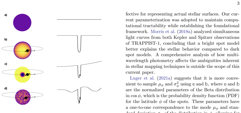
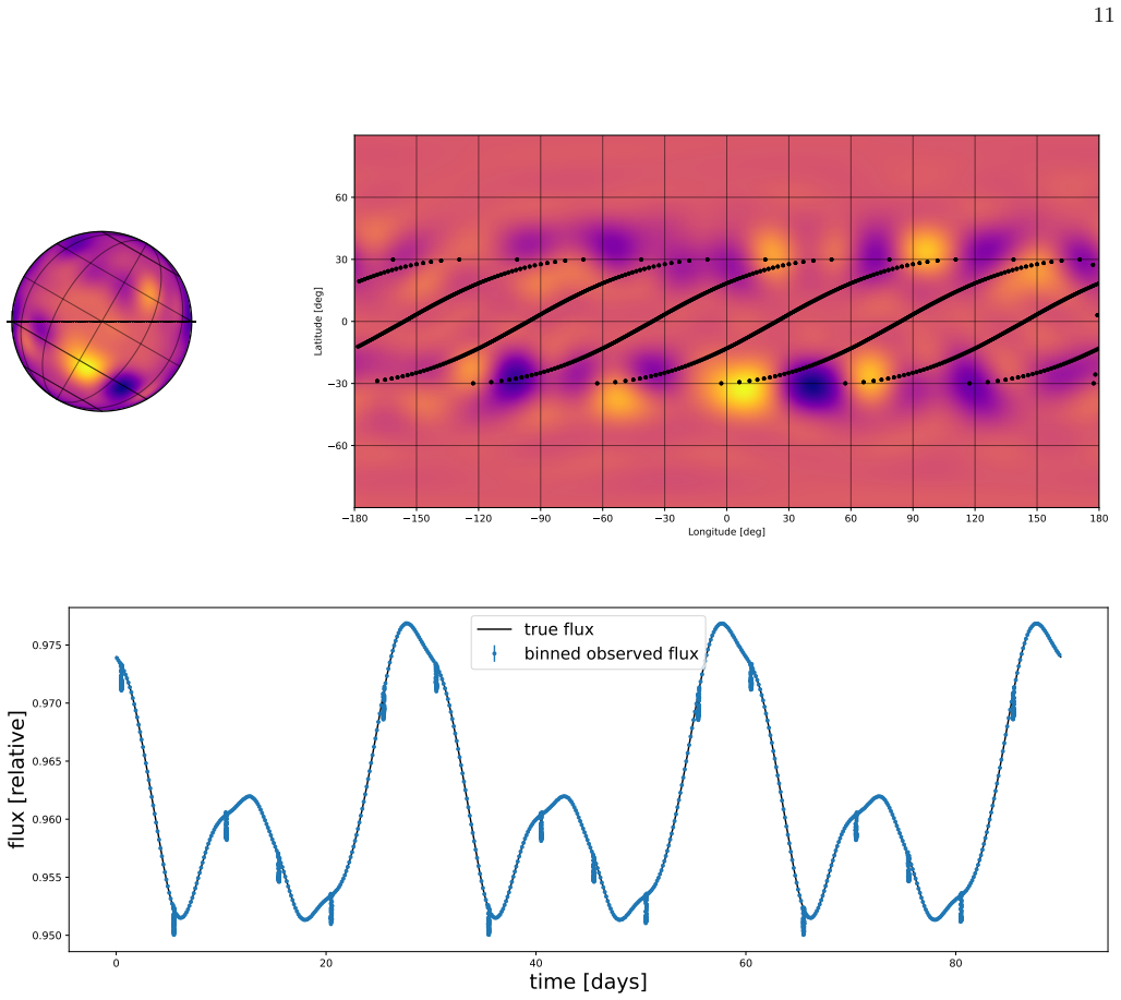
The machinery is the Gaussian-process prior over spherical-harmonic surface coefficients, combined with the linear design matrix that turns a surface map into an observed light curve. The flux is written as $\mathbf{M}(\Theta)\,\mathbf{y}$, so with a Gaussian prior on the map $\mathbf{y}$ the map can be integrated out exactly; the resulting marginal covariance $\mathbf{B} = \mathbf{C} + \mathbf{M}\Lambda\mathbf{M}^\top$ is what the sampler evaluates. Transits enter through the design matrix, so each spot-crossing bump contributes information along the planet's chord rather than only from disk-integrated rotation. A transformed stellar-orientation coordinate system with a half-normal prior breaks the reflection degeneracy between inclination and obliquity during sampling, and the time-dependent extension linearly interpolates between independent surface maps at successive epochs.
What would settle it
Generate synthetic transit light curves from surfaces with large, bright spots of order-unity contrast and run the same inference; if the recovered spot latitude distribution, size, or obliquity shifts outside the quoted uncertainties, the linearity assumption is falsified. Alternatively, multi-band transit photometry of TOI-3884 that resolves whether the crossing feature is bright or dark would directly test whether the near-polar spot interpretation is an artifact of the small-spot linear model.
Extended reading notes
Core claim
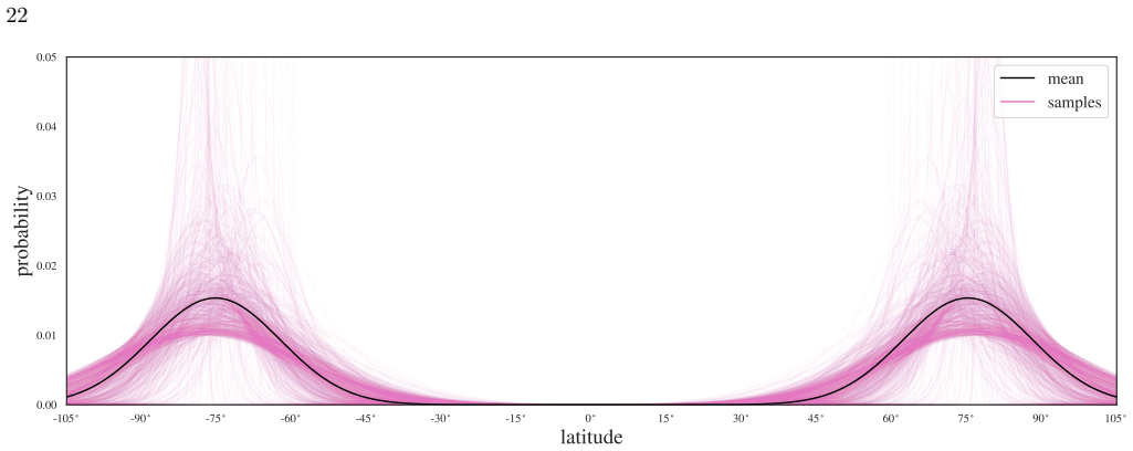
The central discovery is that a Gaussian-process prior on the spherical-harmonic coefficients of a stellar surface, combined with an analytic transit design matrix, lets each transit carve information out of the null space that rotational light curves alone cannot see. Because both the prior and the map-to-flux operation are Gaussian and linear, the surface map can be marginalized analytically, leaving a Gaussian likelihood whose covariance encodes measurement noise plus spot-induced correlated variability. Spot-crossing events then constrain spot latitude, size, contrast, and number, along with stellar inclination and obliquity. For TOI-3884 the model finds spot latitudes concentrated near $\pm 75^\circ$, a stellar inclination of about $35^\circ$, and a sky-projected obliquity near $80^\circ$, with consistency against an independent spectroscopic $v \sin i$ measurement.
Load-bearing premise
The model assumes spot-induced brightness changes are small enough that the flux is linear in the spherical-harmonic surface map, an assumption the paper notes prevents it from distinguishing bright from dark spots; if spots are large or include bright regions, the inferred contrasts, sizes, and the high-latitude reading of TOI-3884 could be biased.
Editorial extensions
If this is right
- Spot latitude distributions can be inferred from single-band transit photometry, not only from rotational modulation, so spot-crossing events become direct diagnostics of stellar magnetic activity.
- Stellar inclination and obliquity can be constrained photometrically, opening spin-orbit studies for faint or otherwise inaccessible systems where high-resolution spectroscopy is impractical.
- Jointly modeling spot crossings with transits reduces stellar contamination in derived planetary radii and transit shapes, supporting more accurate corrections for transmission-spectroscopy measurements.
- The evolving-surface extension can track spot emergence, migration, and dissipation across multiple epochs, relevant to long-baseline surveys and future photometric missions.
- For TOI-3884, the inferred polar spot concentration and near-$80^\circ$ obliquity constitute a photometric signature of spin-orbit misalignment and high-latitude magnetic flux emergence.
Reading between the lines
- If the method scales computationally, archival transit surveys could be mined for spot-latitude demographics, effectively turning exoplanet surveys into stellar-activity surveys.
- Multi-band or spectroscopic transit observations, which make spot contrast wavelength-dependent, could break the paper's noted bright-versus-dark spot ambiguity and tighten the inferred spot sizes and latitudes.
- The same analytic marginalization could be adapted to other linear mapping problems, such as eclipse mapping of binaries or Doppler tomography, wherever a Gaussian prior on the mapped quantity is reasonable.
- The finding that spot-crossing statistics carry obliquity information suggests that future transit surveys could measure spin-orbit misalignment distributions for small planets, complementing traditional Rossiter-McLaughlin measurements.
Signed reviews
Editorial analysis
A structured set of objections, weighed in public.
Referee Report
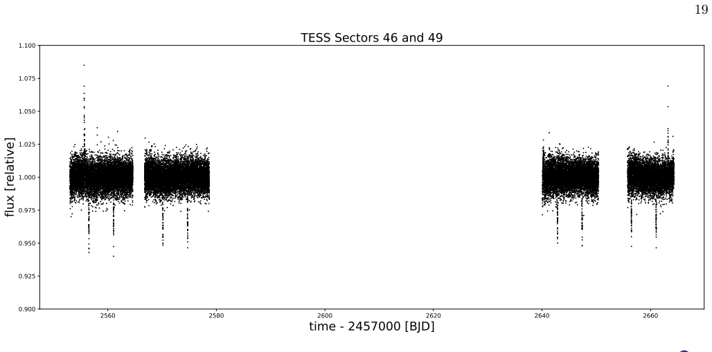
Summary. The paper presents StarryStarryProcess, a hierarchical Bayesian framework that combines the spherical-harmonic surface representation of starry with the Gaussian-process spot model of StarryProcess and a full transit model, in order to infer stellar surface features, stellar inclination, obliquity, and spot parameters from transit light curves. The surface map is marginalized analytically, leaving a Gaussian-process likelihood over the hyperparameters. The authors validate the framework with two synthetic experiments (a static surface and an evolving surface), recovering input parameters within roughly 2σ and illustrating the inclination–obliquity reflection degeneracy. They then apply the model to TESS observations of TOI-3884 and report a high-latitude spot concentration (µϕ ≈ 75°), a low stellar inclination (i⋆ ≈ 35°), and a large spin-orbit obliquity (ψ⋆ ≈ 80°). Section 5.2 claims that the photometrically derived v sin i provides strong independent validation of the geometric model. The paper has a reproducibility appendix, with code, data, and notebooks linked from the figures.
Significance. If the method is sound, the paper makes a useful methodological contribution: it extends the starry/StarryProcess framework to the transit-occultation geometry, shows that spot latitude, stellar inclination, and obliquity can in principle be constrained from single-band photometry, and demonstrates the approach on a real TESS target. The analytical marginalization of the surface map is elegant, the synthetic experiments are clearly described, and the reproducibility infrastructure (public code, chains, and notebooks) is a genuine strength. The central limitation is that the synthetic tests draw data from the same model family and therefore do not independently validate the TOI-3884 inferences; the claimed external validation through v sin i is, as written, internally inconsistent. The paper's significance for stellar-activity and obliquity studies depends on resolving that inconsistency and on clarifying the latitude-parameterization issue.
major comments (4)
- [Table 2, §5.2, Figure 22] The manuscript reports three mutually incompatible values for the photometrically derived v sin i of TOI-3884: Table 2 gives 1.69+0.11−0.09 km/s, §5.2 states 'v sini⋆ = 5.2+0.7−0.8 km/s' and calls this 'strong independent validation', and the text around Figure 22 says 'approximately 2.5 km/s'. These cannot all be summaries of the same posterior. The comparison with the spectroscopic value of 3.59 ± 0.92 km/s from Libby-Roberts et al. (2023) is therefore not a validation; depending on which number is used, the photometric result sits on different sides of the spectroscopic measurement. Because v sin i is the principal external check on the photometrically recovered stellar inclination and obliquity, the TOI-3884 geometric claims need to be recomputed with a single, correctly defined conversion from P⋆ and i⋆, and the stellar radius used in that conversion must be stated consistently with §4.1.
- [Table 2, §5.2, §4.1] The rotation period reported in Table 2, P⋆ = 9.07+0.45−0.51 d, is in strong tension with the Libby-Roberts et al. (2023) entry quoted in the same table, P⋆ < 4.22 ± 1.09 d, yet the discussion does not address this discrepancy. The rotation period and inclination jointly enter the v sin i derivation and the interpretation of spot latitudes, so a >2σ disagreement with an independent measurement is load-bearing and must be discussed, not omitted. Relatedly, §4.1 states that the stellar radius is fixed at 1 R☉; this is inconsistent with the inferred stellar density ρ⋆ = 15.18 g cm⁻³, which would correspond to a star of roughly 10.8 M☉ at 1 R☉. The radius assumption (or the sentence describing it) needs to be corrected, since the derived v sin i and the geometric interpretation depend directly on it.
- [Section 2, Eqs. (3)–(7)] The latitude parameterization is defined through a Beta distribution on cosϕ, but Eqs. (6)–(7) identify µϕ and σ²ϕ with the mean and variance of a Beta random variable. For a random variable X = cosϕ, E[X] = α/(α+β) and Var[X] = αβ/((α+β)²(α+β+1)) are the mean and variance of cosϕ, not of the latitude ϕ. The text also refers to a 'mode' of the latitude distribution, which would have yet another formula. As written, the quoted TOI-3884 result 'µϕ = 75.24°' is therefore not the mean spot latitude under the stated model, and the interpretation of a near-polar spot is ambiguous until the correct mapping from (µϕ, σϕ) to (α, β) is supplied and used consistently in the figures and tables.
- [Section 3.2, Table 1] The synthetic experiments are self-consistency checks: the data are generated from the same StarryProcess prior and the same starry design matrix used for the inference, and the TOI-3884 analysis is the only independent test. Given that the v sin i validation in §5.2 is inconsistent, the paper currently lacks an out-of-sample check that would justify the claim that transit photometry alone can reliably recover stellar orientation and spot latitudes. The authors should either add a test with data drawn from a different generative model (for example, discrete circular spots, or a surface not obeying the GP prior) or explicitly restrict the validation claim to self-consistency.
minor comments (4)
- [Section 3.1] The prior on the planetary inclination is written as U(−bmax,−bmax); it should read U(−bmax, bmax).
- [Throughout] There are several typos that should be corrected in a revision: 'simultaniously' (§1), 'beacuse' (§2), 'distiguish' (§2), 'Firgure' (§3.3), 'imroved' (§5.3), and 'T able 1' in the Table 1 caption.
- [Appendix A] The reproducibility software is cited as 'show your work! (?)'; the placeholder question mark should be replaced with a proper citation or a clear description of the tool.
- [Section 2.3] The sentence 'yi+1 does not depend on yi−1' is confusing in the context of linear interpolation; the authors should clarify that the prior on each map is independent even though consecutive maps are interpolated between epochs.
Circularity Check
No significant circularity: the photometric inversion is a genuine fit with broad priors, and the synthetic tests are calibration checks rather than construction-forced predictions.
full rationale
The model's core relation f_true = M(Theta)y (Eq. 10) with a Gaussian prior on y makes the marginal likelihood (Eq. 13) an ordinary GP likelihood; the spherical-harmonic prior is taken from Luger et al. (2021a), but that is a published model/algorithm used as a component, not a self-citation invoked to forbid alternatives or to establish the target result. No equation defines the inferred spot parameters in terms of the claimed outputs: mu_phi, sigma_phi, n, c, and r are hyperparameters of the Beta/GP prior and are constrained by the transit light curve through Eq. 13. The synthetic experiments draw a true map from the same process and then fit it; the paper explicitly frames this as calibration ('To verify the proper calibration of our model'), and a recovery test can fail (indeed n and c show a known degeneracy), so it is not a prediction forced by construction. For TOI-3884, the priors are broad (e.g., mu_phi ~ U(0.1, 80), P_star from 2 to 18 d), and the high-latitude posterior is data-driven rather than hard-wired. The v sin i comparison is an external check against Libby-Roberts et al. (2023) spectroscopy, not a fitted parameter renamed as a prediction; the fact that Section 5.2, Table 2, and Figure 22 report mutually inconsistent v sin i values is an internal-consistency/correctness problem, not a circularity. Consequently no step in the derivation reduces by construction to its inputs, and the central claim retains independent content.
Assumptions & free parameters
free parameters (5)
- n (number of spots) =
7.58 (+1.39/-2.85) for TOI-3884; 4.45 (+3.53/-2.6) in synthetic Experiment I
- c (spot contrast) =
0.049 (+0.028/-0.013) for TOI-3884
- r (spot angular radius) =
26.77 (+9.7/-8.7) degrees for TOI-3884
- mu_phi (mean spot latitude) =
75.24 (+2.67/-4.11) degrees for TOI-3884
- sigma_phi (latitude spread) =
12.99 (+4.91/-5.08) degrees for TOI-3884
assumptions (6)
- domain assumption The stellar surface brightness map has a Gaussian process prior in spherical harmonic space with covariance from StarryProcess.
- domain assumption The observed flux is a linear function of the surface map via the starry design matrix.
- ad hoc to paper Spot-induced brightness changes are small, so the linear approximation holds and bright and dark spots cannot be distinguished.
- domain assumption Spot latitudes follow a Beta distribution in cos(latitude).
- domain assumption The stellar radius is fixed to 1 R_sun for TOI-3884.
- domain assumption For evolving surfaces, maps at different epochs are linearly interpolated, with each map a fresh draw from the same GP prior.
Cite this review
Pith. "Pith review of Polka-dotted Stars: a Hierarchical Model for Mapping Stellar Surfaces Using Occultation Light Curves and the Case of TOI-3884." pith.science (2026). https://pith.science/paper/TCCHL4AW
@misc{pith2026250421852,
  author       = {Pith},
  title        = {Pith review of: Polka-dotted Stars: a Hierarchical Model for Mapping Stellar Surfaces Using Occultation Light Curves and the Case of TOI-3884},
  year         = {2026},
  howpublished = {\url{https://pith.science/paper/TCCHL4AW}},
  note         = {Machine review of arXiv:2504.21852}
}
read the original abstract
We present StarryStarryProcess, a novel hierarchical Bayesian framework for mapping stellar surfaces using exoplanet transit light curves. While previous methods relied solely on stellar rotational light curves -- which contain limited information about spot properties -- our approach leverages planetary transits as probes of stellar surfaces. When a planet crosses a spot during transit, it creates a distinctive change in the light curve that directly reveals spot properties. Our model integrates planetary transit modeling with stellar variability analysis by combining the spherical harmonic surface map representation from starry, the probabilistic approach to spot properties of StarryProcess, and a comprehensive transit model that accounts for spot-crossing events during transits. We demonstrate through synthetic data experiments that our model successfully recovers spot distributions, stellar orientation, and spot physical properties. We extend the framework to handle evolving stellar surfaces through time-dependent modeling. Applying our method to TESS observations of TOI-3884, we find evidence for high-latitude spot concentrations and significant spin-orbit misalignment. The transit-based approach overcomes fundamental limitations of previous models by providing constraints on spot properties that would remain hidden in the null space of rotational light curves alone. This methodology enables more accurate exoplanet characterization by disentangling stellar activity due to starspots from planetary signals while simultaneously providing insights into stellar magnetic activity patterns. The whole paper is reproducible, and can be found by clicking the GitHub icon.
Figures


Figures from the paper (19 more)







Forward citations
Cited by 1 Pith paper
-
Spot-Crossing Variations Confirm a Misaligned Orbit for a Planet Transiting an M Dwarf
Photometry and transit-shape modeling of TOI-3884 reveal an 11-day stellar rotation period and a polar starspot, confirming a misaligned orbit (true obliquity about 77 degrees) for the hot Neptune TOI-3884 b.
Reference graph
Works this paper leans on
-
[1]
M., Bonfils, X., Forveille, T., et al
Almenara, J. M., Bonfils, X., Forveille, T., et al. 2022, A&A, 667, L11, doi: 10.1051/0004-6361/202244791
-
[2]
Barnes, J. R., Jeffers, S. V., Haswell, C. A., et al. 2017, MNRAS, 471, 811, doi: 10.1093/mnras/stx1482 B´ eky, B., Kipping, D. M., & Holman, M. J. 2014, MNRAS, 442, 3686, doi: 10.1093/mnras/stu1061
-
[3]
2006, A&A, 446, 1027, doi: 10.1051/0004-6361:20042475
Chabrier, G., & K¨ uker, M. 2006, A&A, 446, 1027, doi: 10.1051/0004-6361:20042475
-
[4]
Duane, S., Kennedy, A. D., Pendleton, B. J., & Roweth, D. 1987, Physics Letters B, 195, 216, doi: 10.1016/0370-2693(87)91197-X
-
[5]
Ducrot, E., Sestovic, M., Morris, B. M., et al. 2018, AJ, 156, 218, doi: 10.3847/1538-3881/aade94
-
[6]
Earl, D. J., & Deem, M. W. 2005, Physical Chemistry Chemical Physics, 7, 3910, doi: 10.1039/b509983h
doi:10.1039/b509983h 2005
-
[7]
Foreman-Mackey, D., Hogg, D. W., Lang, D., & Goodman, J. 2013, PASP, 125, 306, doi: 10.1086/670067
doi:10.1086/670067 2013
-
[8]
2013, A&A, 549, L5, doi: 10.1051/0004-6361/201220317
Gastine, T., Morin, J., Duarte, L., et al. 2013, A&A, 549, L5, doi: 10.1051/0004-6361/201220317
Show all 36 references
-
[9]
2016, A&A, 586, A131, doi: 10.1051/0004-6361/201425369
Herrero, E., Ribas, I., Jordi, C., et al. 2016, A&A, 586, A131, doi: 10.1051/0004-6361/201425369
2016 doi
- [10]
- [11]
-
[12]
X., Vanderburg, A., P´ al, A., et al
Huang, C. X., Vanderburg, A., P´ al, A., et al. 2020, Research Notes of the AAS, 4, 204, doi: 10.3847/2515-5172/abca2e
2020 doi
-
[13]
F., Czesla, S., Wolter, U., & Schmitt, J
Huber, K. F., Czesla, S., Wolter, U., & Schmitt, J. H. M. M. 2010, A&A, 514, A39, doi: 10.1051/0004-6361/200913914
2010 doi
-
[14]
M., & Jehn, F
Ilin, E., Angus, R., Luger, R., Morris, B. M., & Jehn, F. U. 2023, MNRAS, 523, 4326, doi: 10.1093/mnras/stad1690
2023 doi
-
[15]
J., et al
Ilin, E., Poppenhaeger, K., Schmidt, S. J., et al. 2021, MNRAS, 507, 1723, doi: 10.1093/mnras/stab2159
2021 doi
-
[16]
2016, SPIE Bellingham
Jenkins, J., Chiozzi, G., & Guzman, J. 2016, SPIE Bellingham
2016
-
[17]
G., Lendl, M., Cubillos, P
Juvan, I. G., Lendl, M., Cubillos, P. E., et al. 2018, A&A, 610, A15, doi: 10.1051/0004-6361/201731345
2018 doi
-
[18]
E., Schutte, M., Hebb, L., et al
Libby-Roberts, J. E., Schutte, M., Hebb, L., et al. 2023, AJ, 165, 249, doi: 10.3847/1538-3881/accc2f Lightkurve Collaboration, Cardoso, J. V. d. M., Hedges, C., et al. 2018, Lightkurve: Kepler and TESS time series analysis in Python, Astrophysics Source Code Library. http://a...
2023 doi
-
[19]
2023, ApJL, 955, L22, doi: 10.3847/2041-8213/acf7c4
Lim, O., Benneke, B., Doyon, R., et al. 2023, ApJL, 955, L22, doi: 10.3847/2041-8213/acf7c4
2023 doi
-
[20]
2019, AJ, 157, 64, doi: 10.3847/1538-3881/aae8e5
Luger, R., Agol, E., Foreman-Mackey, D., et al. 2019, AJ, 157, 64, doi: 10.3847/1538-3881/aae8e5
2019 doi
-
[21]
2021a, AJ, 162, 124, doi: 10.3847/1538-3881/abfdb9
Luger, R., Foreman-Mackey, D., & Hedges, C. 2021a, AJ, 162, 124, doi: 10.3847/1538-3881/abfdb9
-
[22]
Luger, R., Foreman-Mackey, D., Hedges, C., & Hogg, D. W. 2021b, AJ, 162, 123, doi: 10.3847/1538-3881/abfdb8
-
[23]
Maxted, P. F. L. 2016, A&A, 591, A111, doi: 10.1051/0004-6361/201628579
2016 doi
-
[24]
2014, MNRAS, 444, 1721, doi: 10.1093/mnras/stu1530 31
Montalto, M., Bou´ e, G., Oshagh, M., et al. 2014, MNRAS, 444, 1721, doi: 10.1093/mnras/stu1530 31
2014 doi
-
[25]
F., Petit, P., et al
Morin, J., Donati, J. F., Petit, P., et al. 2008, MNRAS, 390, 567, doi: 10.1111/j.1365-2966.2008.13809.x
2008
-
[26]
M., Agol, E., Hebb, L., & Hawley, S
Morris, B. M., Agol, E., Hebb, L., & Hawley, S. L. 2018a, AJ, 156, 91, doi: 10.3847/1538-3881/aad3b7 —. 2018b, AJ, 156, 91, doi: 10.3847/1538-3881/aad3b7
-
[27]
Hawley, S. L. 2017, ApJ, 846, 99, doi: 10.3847/1538-4357/aa8555
2017 doi
-
[28]
2013, A&A, 549, A35, doi: 10.1051/0004-6361/201220173
Oshagh, M., Boisse, I., Bou´ e, G., et al. 2013, A&A, 549, A35, doi: 10.1051/0004-6361/201220173
2013 doi
-
[29]
F., et al
Scandariato, G., Nascimbeni, V., Lanza, A. F., et al. 2017, A&A, 606, A134, doi: 10.1051/0004-6361/201730966
2017 doi
-
[30]
Silva, A. V. R. 2003, ApJL, 585, L147, doi: 10.1086/374324
2003 doi
-
[31]
Solanki, S. K. 2003, A&A Rv, 11, 153, doi: 10.1007/s00159-003-0018-4
2003 doi
-
[32]
Strassmeier, K. G. 2009, A&A Rv, 17, 251, doi: 10.1007/s00159-009-0020-6
2009 doi
-
[33]
2013, MNRAS, 428, 3671, doi: 10.1093/mnras/sts306
Tregloan-Reed, J., Southworth, J., & Tappert, C. 2013, MNRAS, 428, 3671, doi: 10.1093/mnras/sts306
2013 doi
-
[34]
2015, MNRAS, 450, 1760, doi: 10.1093/mnras/stv730
Tregloan-Reed, J., Southworth, J., Burgdorf, M., et al. 2015, MNRAS, 450, 1760, doi: 10.1093/mnras/stv730
2015 doi
-
[35]
D., Farr, W
Vousden, W. D., Farr, W. M., & Mandel, I. 2016, MNRAS, 455, 1919, doi: 10.1093/mnras/stv2422
2016 doi
-
[36]
K., Gastine, T., Christensen, U
Yadav, R. K., Gastine, T., Christensen, U. R., & Reiners, A. 2015, A&A, 573, A68, doi: 10.1051/0004-6361/201424589
2015 doi
Reviewed August 16, 2026 · model on record in the stance chip above.
Discussion (0). Continue with ORCID to comment.