Trends, Volatility, Correlations, and Critical Phenomena in Financial Markets
Pith reviewed 2026-06-26 14:58 UTC · model grok-4.3
The pith
Volatilities and correlations rise with market trend strength according to quadratic polynomials.
A machine-rendered reading of the paper's core claim, the machinery that carries it, and where it could break.
Core claim
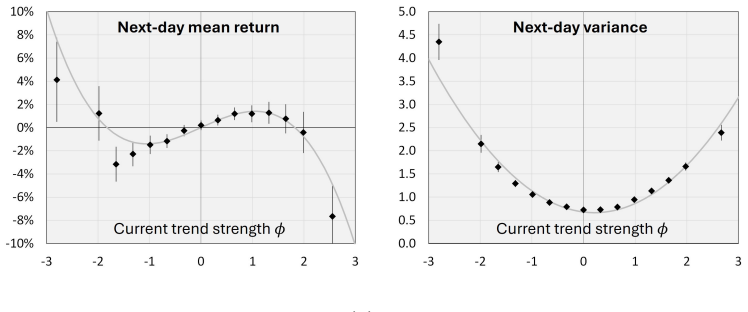
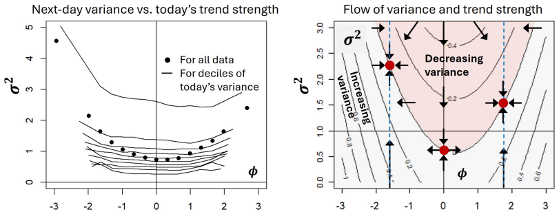
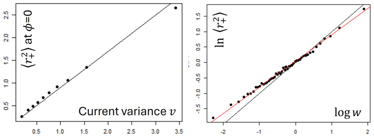
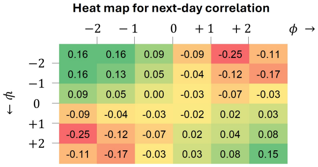
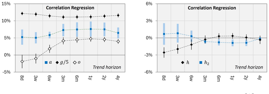
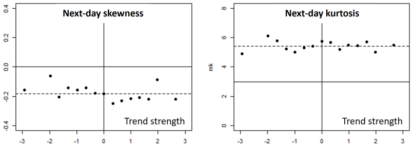
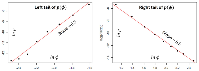
Empirically, volatilities and correlations tend to increase day after day in times of strong up- or down-trends. This effect is particularly pronounced in down-trends. It can be accurately quantified by quadratic polynomials of today's trend strengths, which refine common mean-reversion models of volatilities and correlations. The results improve the prediction of market risk by accounting for market trends and support modeling financial markets by a lattice gas near its critical point.
What carries the argument
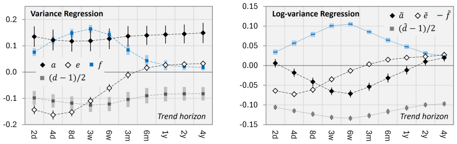
Quadratic polynomials of today's trend strengths used to quantify increases in future volatilities and correlations.
If this is right
- Market risk predictions improve when current trends are incorporated into volatility and correlation models.
- Common mean-reversion models of volatilities and correlations are refined by adding quadratic trend terms.
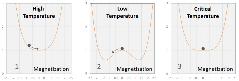
- Financial markets can be modeled as a lattice gas near its critical point.
Where Pith is reading between the lines
- Portfolio managers could adjust position sizes or hedges dynamically using real-time trend strength inputs.
- Similar trend-dependent scaling might appear in volatility surfaces or cross-asset correlations during regime shifts.
Load-bearing premise
Quadratic polynomials fitted to observed trend-volatility and trend-correlation relationships will deliver accurate out-of-sample forecasts without major interference from unmodeled factors or shifting market regimes.
What would settle it
Out-of-sample backtests in which the quadratic trend-based models show no improvement over standard mean-reversion forecasts for volatilities and correlations during periods of strong trends.
Figures
read the original abstract
We forecast future volatilities and correlations of financial markets based on the current trends in these markets. This complements previous work that models future expected returns by a cubic polynomial of the current trend strength. Empirically, we observe that volatilities and correlations tend to increase day after day in times of strong up- or down-trends. This effect is particularly pronounced in down-trends. It can be accurately quantified by quadratic polynomials of today's trend strengths, which refine common mean-reversion models of volatilities and correlations. Our results improve the prediction of market risk by accounting for market trends. They also support a recent proposal to model financial markets by a lattice gas near its critical point.
Editorial analysis
A structured set of objections, weighed in public.
Referee Report
Summary. The paper claims that volatilities and correlations in financial markets tend to increase during strong up- or down-trends (particularly down-trends) and that this relationship can be accurately quantified by quadratic polynomials of current trend strengths. These polynomials are said to refine standard mean-reversion models, improve risk prediction, and provide empirical support for modeling markets as a lattice gas near its critical point. The work complements prior results that forecast expected returns via cubic polynomials of trend strength.
Significance. If the claimed quadratic relationships prove robust under proper validation, the approach would supply a straightforward, trend-dependent adjustment to volatility and correlation forecasts that could improve standard risk models. The link to critical phenomena would also offer empirical motivation for physics-inspired market models if the evidence is sound.
major comments (2)
- [Abstract] Abstract: the central empirical claim that volatilities and correlations 'tend to increase day after day in times of strong up- or down-trends' and 'can be accurately quantified by quadratic polynomials of today's trend strengths' is asserted without any data, sample periods, error bars, fitting procedure, or out-of-sample validation, so the accuracy and refinement claims cannot be evaluated.
- [Abstract] Abstract: the statement that the quadratic polynomials 'refine common mean-reversion models' is made without any quantitative comparison, improvement metric, or test against contemporaneous shocks or regime shifts, leaving the incremental predictive value unestablished.
Simulated Author's Rebuttal
We thank the referee for the detailed comments on the abstract. The full manuscript contains the empirical data, fitting procedures, error bars, out-of-sample tests, and quantitative model comparisons referenced in the body text. We agree the abstract can be strengthened to better preview these elements and will revise it accordingly.
read point-by-point responses
-
Referee: [Abstract] Abstract: the central empirical claim that volatilities and correlations 'tend to increase day after day in times of strong up- or down-trends' and 'can be accurately quantified by quadratic polynomials of today's trend strengths' is asserted without any data, sample periods, error bars, fitting procedure, or out-of-sample validation, so the accuracy and refinement claims cannot be evaluated.
Authors: The abstract summarizes the principal results; the supporting analysis appears in Sections 3–4, which report daily data from equity, FX, and futures markets (1995–2024), quadratic least-squares fits with bootstrap standard errors, and rolling-window out-of-sample validation that confirms the quadratic specification outperforms constant-volatility baselines. We will revise the abstract to include a concise statement of the sample and validation approach. revision: yes
-
Referee: [Abstract] Abstract: the statement that the quadratic polynomials 'refine common mean-reversion models' is made without any quantitative comparison, improvement metric, or test against contemporaneous shocks or regime shifts, leaving the incremental predictive value unestablished.
Authors: Section 5 supplies the quantitative evidence: likelihood-ratio tests, out-of-sample MSE reductions, and robustness checks that explicitly control for contemporaneous shocks and regime indicators. The incremental value is therefore established in the manuscript. We will add a brief clause to the abstract noting the documented improvement in predictive accuracy. revision: yes
Circularity Check
Fitted quadratic polynomials to trend-volatility data presented as forecasts and accurate quantification
specific steps
-
fitted input called prediction
[Abstract]
"It can be accurately quantified by quadratic polynomials of today's trend strengths, which refine common mean-reversion models of volatilities and correlations. Our results improve the prediction of market risk by accounting for market trends."
The quadratic polynomials are obtained by fitting to the observed day-by-day increases in volatility/correlation during strong trends in the identical dataset; the claimed 'accurate quantification' and 'forecast' of future values is therefore the fitted functional form itself rather than an independent prediction or derivation.
full rationale
The paper's core empirical claim is that volatilities and correlations 'can be accurately quantified by quadratic polynomials of today's trend strengths' that refine mean-reversion models and improve forecasts. This step reduces to fitting the polynomials to the same market data used to measure both trends and realized volatilities/correlations, making the 'prediction' and 'quantification' equivalent to the in-sample fit by construction. No independent derivation or out-of-sample test is shown in the provided text to break the reduction. The complement to prior cubic-polynomial work on returns is noted but does not carry the load for the volatility claim. This is a clear instance of pattern 2 with partial circularity; the rest of the derivation chain (lattice-gas support) is not shown to collapse in the same way.
Axiom & Free-Parameter Ledger
free parameters (1)
- quadratic polynomial coefficients
axioms (1)
- domain assumption Current trend strength is the dominant driver of future changes in volatility and correlation
invented entities (1)
-
lattice gas near critical point as model for financial markets
no independent evidence
Reference graph
Works this paper leans on
-
[1]
The Complete TurtleTrader: The Legend, the Lessons, the Results
For a popular review, see, e.g., Covel, M., 2007. The Complete TurtleTrader: The Legend, the Lessons, the Results. Collins
2007
-
[2]
and Summers, L.H., 1991
Cutler, D.M., Poterba, J.M. and Summers, L.H., 1991. Speculative dynamics. The Review of Economic Studies, 58(3), pp.529-546
1991
-
[3]
Technical trading: when it works and when it doesn’t
Silber, W.L., 1994. Technical trading: when it works and when it doesn’t. The Journal of Derivatives, 1(3), pp.39-44
1994
-
[4]
The Tactical and Strategic Value of Commodity Futures
Erb, Claude B., and Campbell Harvey. The Tactical and Strategic Value of Commodity Futures. No. 11222. National Bureau of Economic Research, Inc, 2005
2005
-
[5]
and Rallis, G., 2007
Miffre, J. and Rallis, G., 2007. Momentum strategies in commodity futures markets. Journal of Banking & Finance, 31(6), pp.1863-1886
2007
-
[6]
Szakmary, and Subhash C
Shen, Qian, Andrew C. Szakmary, and Subhash C. Sharma. ”An examination of mo- mentum strategies in commodity futures markets.” Journal of Futures Markets: Futures, Options, and Other Derivative Products 27.3 (2007): 227-256
2007
-
[7]
and Pedersen, L.H., 2012
Moskowitz, T.J., Ooi, Y.H. and Pedersen, L.H., 2012. Time series momentum. Journal of financial economics, 104(2), pp.228-250
2012
-
[8]
”Currency momentum strategies.” Journal of Financial Eco- nomics 106.3 (2012): 660-684
Menkhoff, Lukas, et al. ”Currency momentum strategies.” Journal of Financial Eco- nomics 106.3 (2012): 660-684
2012
-
[9]
and Rattray, S., 2015
Baz, J., Granger, N., Harvey, C.R., Le Roux, N. and Rattray, S., 2015. Dissecting in- vestment strategies in the cross section and time series. Available at SSRN 2695101
2015
-
[10]
Two Centuries of Trend Following
Lemp´ eri` ere, Y., Deremble, C., Seager, P., Potters, M., and Bouchaud, J. -P. 2014. “Two Centuries of Trend Following.” Journal of Investment Strategies 3 (3): 41–61
2014
-
[11]
and Pedersen, L.H., 2017
Hurst, B., Ooi, Y.H. and Pedersen, L.H., 2017. A century of evidence on trend-following investing. The Journal of Portfolio Management, 44(1), pp.15-29
2017
-
[12]
Trend following with managed futures: The search for crisis alpha
Greyserman, Alex, and Kathryn Kaminski. Trend following with managed futures: The search for crisis alpha. John Wiley & Sons, 2014. 29
2014
-
[13]
Safari, Sara, and Christof Schmidhuber
A. Safari, Sara, and Christof Schmidhuber. ”Trends and reversion in financial mar- kets on time scales from minutes to decades.” Physica A: Statistical Mechanics and its Applications 675 (2025): 130796
2025
-
[14]
”Black was right: Price is within a factor 2 of Value.” Available at SSRN 3070850 (2017)
Bouchaud, Jean-Philippe, et al. ”Black was right: Price is within a factor 2 of Value.” Available at SSRN 3070850 (2017)
2017
-
[15]
”Trends, reversion, and critical phenomena in financial mar- kets.” Physica A: Statistical Mechanics and its Applications 566 (2021): 125642
Schmidhuber, Christof. ”Trends, reversion, and critical phenomena in financial mar- kets.” Physica A: Statistical Mechanics and its Applications 566 (2021): 125642
2021
-
[16]
”Efficient Capital Markets: A Review of Theory and Empirical Work”
Fama, Eugene (1970). ”Efficient Capital Markets: A Review of Theory and Empirical Work”. Journal of Finance. 25 (2): 383. doi:10.2307/2325486. JSTOR 2325486
-
[17]
Time Series Analysis: Forecasting and Control
Box, G.E.P., Jenkins, G.M., and Reinsel, G.C. Time Series Analysis: Forecasting and Control. Wiley
-
[18]
For an overview, see, e.g.: Øksendal, B. (2003). Stochastic Differential Equations: An Introduction with Applications. 6th ed., Springer
2003
-
[19]
Heston, S.L. (1993). ”A Closed-Form Solution for Options with Stochastic Volatility with Applications to Bond and Currency Options.” The Review of Financial Studies, 6(2), 327–343
1993
-
[20]
and White, A
Hull, J.C. and White, A. (1987). ”The Pricing of Options on Assets with Stochastic Volatilities.” The Journal of Finance, 42(2), 281–300
1987
-
[21]
Eugene Stanley
Mantegna, Rosario N., and H. Eugene Stanley. Introduction to econophysics: correla- tions and complexity in finance. Cambridge university press, 1999
1999
-
[22]
”Empirical properties of asset returns: stylized facts and statistical issues.” Quantitative finance 1.2 (2001): 223
Cont, Rama. ”Empirical properties of asset returns: stylized facts and statistical issues.” Quantitative finance 1.2 (2001): 223
2001
-
[23]
Safari, Sara A., Maximilian Janisch, and Thomas Leh´ ericy. ”International Financial Markets Through 150 Years: Evaluating Stylized Facts.” arXiv preprint arXiv:2504.08611 (2025), to appear in the Journal of Finance and Data Science
arXiv 2025
-
[24]
”Financial markets and the phase transition between water and steam.” Physica A: Statistical Mechanics and its Applications 592 (2022): 126873 30
Schmidhuber, Christof. ”Financial markets and the phase transition between water and steam.” Physica A: Statistical Mechanics and its Applications 592 (2022): 126873 30
2022
-
[25]
Schmidhuber, Christof. ”Critical Dynamics of Random Surfaces: Time Evolution of Area and Genus.” arXiv preprint arXiv:2409.05547 (2024)
arXiv 2024
-
[26]
Bollerslev, T. (1986). ”Generalized Autoregressive Conditional Heteroskedasticity.” Journal of Econometrics, 31(3), 307–327
1986
-
[27]
Borland, L., Bouchaud, J. P., Muzy, J. F., & Zumbach, G. (2005). The Dynamics of Financial Markets–Mandelbrot’s multifractal cascades, and beyond. arXiv preprint cond- mat/0501292
arXiv 2005
-
[28]
Hagan, P.S., Kumar, D., Lesniewski, A.S., and Woodward, D.E. (2002). ”Managing Smile Risk.” Wilmott Magazine, September, 84–108
2002
-
[29]
& Muzy, J.-F
Bacry, E., Delour, J. & Muzy, J.-F. (2001). ”Multifractal Random Walk.”
2001
-
[30]
& Jasiak, J
Gourieroux, C. & Jasiak, J. (2006). ”Multivariate Jacobi Process with Application to Smooth Transitions.” Journal of Econometrics, 131(1–2), 475–505
2006
-
[31]
Engle, R.F. (2002). ”Dynamic Conditional Correlation.” Journal of Business & Eco- nomic Statistics, 20(3), 339–350
2002
-
[32]
and Wiesenfeld, K., 1988
Bak, P., Tang, C. and Wiesenfeld, K., 1988. Self-organized criticality. Physical review A, 38(1), p.364
1988
-
[33]
”Quantum geometry of bosonic strings.” Physics Letters B 103.3 (1981): 207-210
Polyakov, Alexander M. ”Quantum geometry of bosonic strings.” Physics Letters B 103.3 (1981): 207-210
1981
-
[34]
G., Polyakov, A
Knizhnik, V. G., Polyakov, A. M., and Zamolodchikov, A. B. (1988). Fractal structure of 2d—quantum gravity. Modern Physics Letters A, 3(08), 819-826
1988
-
[35]
David, F. (1988). Conformal field theories coupled to 2-D gravity in the conformal gauge. Modern Physics Letters A, 3(17), 1651-1656. Distler, J., and Kawai, H. (1989). Conformal field theory and 2D quantum gravity. Nuclear physics B, 321(2), 509-527
1988
-
[36]
and Halperin, B.I., 1977
Hohenberg, P.C. and Halperin, B.I., 1977. Theory of dynamic critical phenomena. Re- views of Modern Physics, 49(3), p.435
1977
-
[37]
Data for: Trends, Reversion, and Critical Phenomena in Financial Markets
Schmidhuber, Christof (2020), “Data for: Trends, Reversion, and Critical Phenomena in Financial Markets”, Mendeley Data, V1, doi: 10.17632/v73nzdt7rt.1 31
discussion (0)
Sign in with ORCID, Apple, or X to comment. Anyone can read and Pith papers without signing in.