REVIEW 2 major objections 2 minor 31 references
STEP: Learning STructured Embeddings for Progressive Time Series
T0 review · 2 major / 2 minor · reviewed 2026-06-28 · grok-4.3
Pith's one-line read A contrastive method embeds progressive time series so the polar angle in latent space tracks irreversible state progression without labels.
desk verdict The orthogonal prototypes create a latent compass where angle tracks progression, and the linear regressor result is the strongest evidence offered, but the contrastive loss may not force monotonic theta without extra terms. read the letter →
The pith
A machine-rendered reading of the paper's core claim, the machinery that carries it, and where it could break.
The reading
What carries the argument
The latent compass formed by polar coordinates (θ, r) derived from the position relative to two fixed orthogonal prototype vectors in the learned embedding space.
What would settle it
Observing that on held-out progressive time series the angle θ shows no correlation with actual progression stages or that linear prediction error exceeds that of black-box models would falsify the claim.
Extended reading notes
Core claim
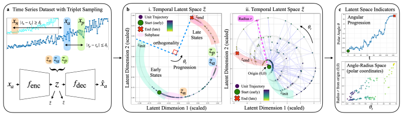
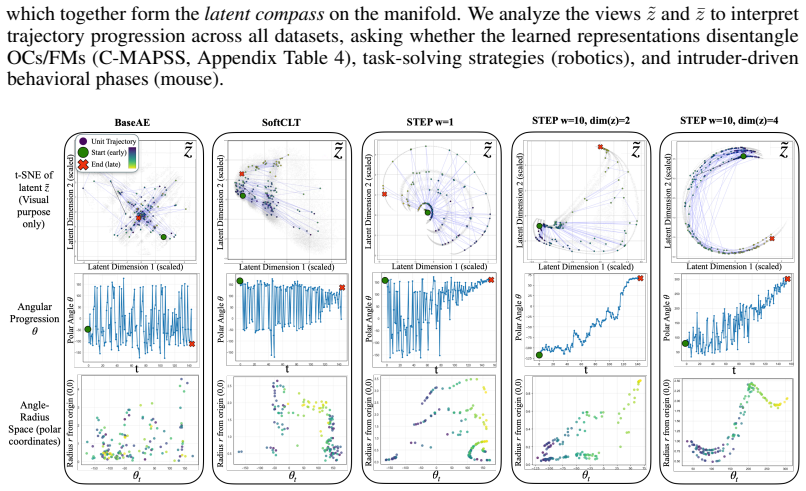
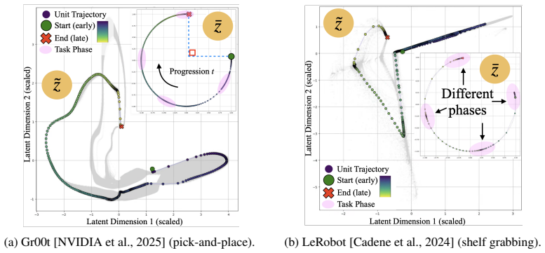
By training with a contrastive objective anchored at two orthogonal prototypes, the method produces a latent manifold whose geometry directly encodes state progression through polar angle, allowing transparent multi-step forecasting and phase identification across industrial, robotic, and neural datasets.
Load-bearing premise
The self-supervised contrastive loss with fixed orthogonal prototypes produces a manifold where polar angle reliably corresponds to state progression in varied domains.
Signed reviews
Editorial analysis
A structured set of objections, weighed in public.
Referee Report
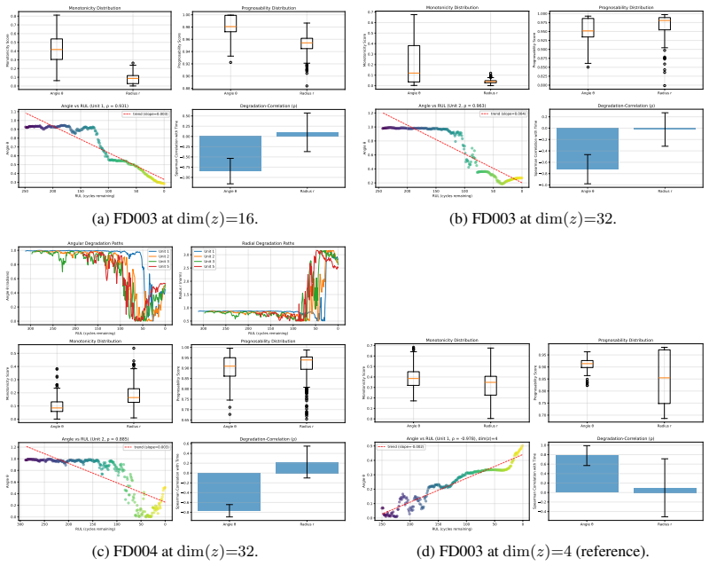
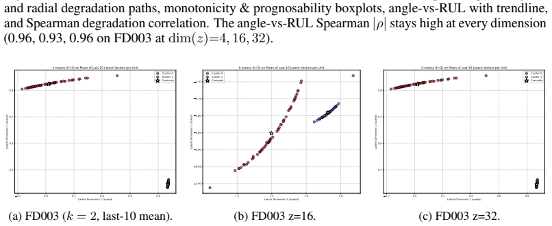
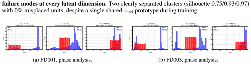
Summary. The paper introduces STEP, a self-supervised contrastive method for progressive time series that embeds observations on a manifold anchored by two fixed orthogonal prototype vectors. From the resulting latent vectors it extracts polar coordinates (θ, r) in which θ is asserted to track irreversible state progression (e.g., healthy to failed) and r identifies the active mode, without proxy labels. The approach is evaluated on industrial degradation, robotic tasks, and neural activity data for end-state prediction, multi-step forecasting, and interpretable phase separation, claiming to match or exceed black-box baselines while a simple linear regressor on the compass coordinates remains competitive.
Significance. If the geometry reliably encodes monotonic progression, the method supplies a transparent, label-free alternative to black-box models for domains where state irreversibility matters. The reported competitiveness of a linear regressor on (θ, r) would constitute direct quantitative evidence that the learned manifold makes the underlying state geometrically accessible.
major comments (2)
- [§3] §3 (contrastive objective): the loss is described as standard contrastive with two fixed orthogonal prototypes, yet no temporal-ordering, monotonicity, or progression-aware term is introduced. Without such a mechanism it is not obvious why θ must align with irreversible state rather than with orthogonal factors; the central claim that θ tracks progression therefore rests on an unproven inductive bias.
- [§4.2, Table 2] §4.2 and Table 2 (linear-regressor experiments): the competitiveness of the linear model on (θ, r) is load-bearing for the interpretability claim, but the manuscript does not report whether prototype vectors or the polar-angle definition were tuned post-hoc on the test set or whether the same linear head was compared against equivalently tuned deep baselines; this leaves open the possibility that the reported performance advantage is an artifact of evaluation choices.
minor comments (2)
- [Abstract, §2] Notation for the polar coordinates is introduced as ({ heta}, r) in the abstract but later appears without braces; consistent typesetting would aid readability.
- [§4.1] Dataset sizes, sampling rates, and exact train/validation/test splits are not tabulated; these details are needed to assess whether the reported forecasting horizons are comparable across domains.
Simulated Author's Rebuttal
We thank the referee for the constructive feedback. Below we address the two major comments point by point, clarifying the inductive bias of the contrastive objective and the evaluation protocol for the linear regressor. We are prepared to revise the manuscript accordingly.
read point-by-point responses
-
Referee: [§3] the loss is described as standard contrastive with two fixed orthogonal prototypes, yet no temporal-ordering, monotonicity, or progression-aware term is introduced. Without such a mechanism it is not obvious why θ must align with irreversible state rather than with orthogonal factors; the central claim that θ tracks progression therefore rests on an unproven inductive bias.
Authors: We agree that the contrastive loss contains no explicit monotonicity or ordering term. The inductive bias arises instead from the geometry: the two prototypes are fixed as orthogonal anchors representing the start and end of the irreversible process, and the contrastive objective (pulling same-trajectory positives toward their nearest prototype while pushing negatives away) encourages trajectories to traverse the manifold along the angular direction. Because the data consist of progressive sequences, this geometry induces θ to correlate with state advancement. We will expand §3 with a dedicated paragraph deriving this bias from the prototype construction and loss geometry, and we will add a short ablation confirming that random (non-orthogonal) prototypes degrade the progression signal. revision: yes
-
Referee: [§4.2, Table 2] the competitiveness of the linear model on (θ, r) is load-bearing for the interpretability claim, but the manuscript does not report whether prototype vectors or the polar-angle definition were tuned post-hoc on the test set or whether the same linear head was compared against equivalently tuned deep baselines; this leaves open the possibility that the reported performance advantage is an artifact of evaluation choices.
Authors: The two prototype vectors are fixed once at initialization as the standard basis vectors e1 and e2 and are never updated or selected on any test data. Polar coordinates are obtained by the deterministic transformation (θ, r) = atan2(v·e2, v·e1), ||v|| with no learned parameters or test-set tuning. The linear regressor is trained solely on the training split using the identical cross-validation protocol applied to all deep baselines. We will add an explicit statement of these choices in §4.2 together with a supplementary table confirming that the linear head was not given any hyper-parameter advantage over the deep models. revision: yes
Circularity Check
No circularity: self-supervised geometry yields independent empirical claims
full rationale
The derivation relies on a self-supervised contrastive objective with fixed orthogonal prototypes to induce a latent manifold whose polar coordinates are then interpreted as tracking progression. No equations or claims in the abstract reduce the reported predictions (end-state prediction, forecasting, phase separation) or the linear-regressor competitiveness result to quantities defined by construction from fitted hyperparameters or prototype choices. No self-citations, uniqueness theorems, or ansatzes imported from prior author work are invoked as load-bearing. The central claim is supported by cross-domain empirical validation rather than algebraic identity with the input loss, satisfying the criteria for a self-contained, non-circular derivation.
Assumptions & free parameters
Cite this review
Pith. "Pith review of STEP: Learning STructured Embeddings for Progressive Time Series." pith.science (2026). https://pith.science/paper/TNYQZBOM
@misc{pith2026260531061,
  author       = {Pith},
  title        = {Pith review of: STEP: Learning STructured Embeddings for Progressive Time Series},
  year         = {2026},
  howpublished = {\url{https://pith.science/paper/TNYQZBOM}},
  note         = {Machine review of arXiv:2605.31061}
}
read the original abstract
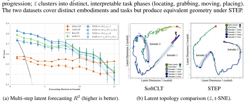
We present a novel method for learning interpretable representations of progressive time series, that is, data capturing irreversible state transitions such as degradation or task completion. Our approach uses a self-supervised contrastive objective to learn a low-dimensional latent space whose geometry is itself the interpretation: each observation becomes a point on a manifold anchored between two fixed orthogonal prototype vectors, and a trajectory becomes a path across that manifold. From this structure we read a latent compass, the polar coordinates ({\theta}, r) of the latent vector, in which {\theta} tracks the progression of the underlying state (e.g., from healthy to failed) and r identifies the active mode (e.g., the operating condition), without any proxy labels. We evaluate the approach against the state of the art on diverse domains, including industrial degradation, robotic tasks, and neural activity, validating three key capabilities: (1) end-state prediction, (2) multi-step forecasting, and (3) interpretable phase separation. Our method matches or improves over black-box counterparts on all of these while providing transparency about the underlying mechanisms. A simple linear regressor on top of the latent compass coordinates is competitive with deep architectures, direct quantitative evidence that the underlying state is encoded in a geometrically accessible form.
Figures
Figures from the paper (12 more)
Reference graph
Works this paper leans on
-
[1]
LeJEPA: Provable and Scalable Self-Supervised Learning Without the Heuristics
Randall Balestriero and Yann LeCun. Lejepa: Provable and scalable self-supervised learning without the heuristics.arXiv preprint arXiv:2511.08544,
-
[2]
LeJEPA: Provable and Scalable Self-Supervised Learning Without the Heuristics
doi: 10.48550/arXiv.2511.08544. Mustafa Gokce Baydogan and George Runger. Time series representation and similarity based on local autopatterns.Data Mining and Knowledge Discovery, 30(2):476–509,
-
[3]
Omar Bougacha, Christophe Varnier, and Noureddine Zerhouni
doi: 10.1162/089976698300017953. Omar Bougacha, Christophe Varnier, and Noureddine Zerhouni. A review of post-prognostics decision-making in prognostics and health management.International Journal of Prognostics and Health Management, 11(15):31,
-
[4]
Semi-supervised end-to-end contrastive learning for time series classification
Huili Cai, Xiang Zhang, and Xiaofeng Liu. Semi-supervised end-to-end contrastive learning for time series classification. (arXiv:2310.08848), March
-
[5]
Semi-supervised end-to-end contrastive learning for time series classification
doi: 10.48550/arXiv.2310.08848. URL http://arxiv.org/abs/2310.08848. arXiv:2310.08848 [cs]. Qianzhong Chen, Justin Yu, Mac Schwager, Pieter Abbeel, Yide Shentu, and Philipp Wu. Sarm: Stage-aware reward modeling for long horizon robot manipulation. (arXiv:2509.25358), Oc- tober
-
[6]
SARM: Stage-Aware Reward Modeling for Long Horizon Robot Manipulation
doi: 10.48550/arXiv.2509.25358. URL http://arxiv.org/abs/2509.25358. arXiv:2509.25358 [cs]. Ting Chen, Simon Kornblith, Mohammad Norouzi, and Geoffrey Hinton. A simple framework for contrastive learning of visual representations. InInternational Conference on Machine Learning (ICML),
-
[7]
Aircraft engine health monitoring using self-organizing maps
Etienne Côme, Marie Cottrell, Michel Verleysen, and Jérôme Lacaille. Aircraft engine health monitoring using self-organizing maps. In10th Industrial Conference, ICDM 2010,, volume 6171, pages 405–417. Springer,
2010
-
[8]
doi: 10.1016/j.ress.2022.108353
ISSN 09518320. doi: 10.1016/j.ress.2022.108353. URL https://linkinghub.elsevier. com/retrieve/pii/S0951832022000321. Ingeborg De Pater and Mihaela Mitici. Novel metrics to evaluate probabilistic remaining useful life prognostics with applications to turbofan engines.PHM Society European Conference, 7(1): 96–109, June
Show all 31 references
-
[9]
doi: 10.36001/phme.2022.v7i1.3320
ISSN 2325-016X, 2325-016X. doi: 10.36001/phme.2022.v7i1.3320. URL https://papers.phmsociety.org/index.php/phme/article/view/3320. Emadeldeen Eldele, Mohamed Ragab, Zhenghua Chen, Min Wu, Chee Keong Kwoh, Xiaoli Li, and Cuntai Guan. Time-series representation learning via tempo...
2022 doi
-
[10]
ISBN 979-8-3503-5401-0
IEEE. ISBN 979-8-3503-5401-0. doi: 10.1109/PHM-Beijing63284.2024.10874536. URLhttps://ieeexplore.ieee.org/document/10874536/. 10 Olga Fink, Qin Wang, Markus Svensén, Pierre Dersin, Wan-Jui Lee, and Melanie Ducoffe. Potential, challenges and future directions for deep learning ...
2024 doi
-
[11]
doi: 10.1016/j.engappai.2020.103678
ISSN 09521976. doi: 10.1016/j.engappai.2020.103678. URL https://linkinghub.elsevier.com/retrieve/ pii/S0952197620301184. Ying Fu, Ye Kwon Huh, and Kaibo Liu. Degradation modeling and prognostic analysis under unknown failure modes.IEEE Transactions on Automation Science and En...
2020 doi
-
[12]
doi: 10.1016/j.ymssp.2013.06.004
ISSN 08883270. doi: 10.1016/j.ymssp.2013.06.004. URL https://linkinghub.elsevier.com/retrieve/ pii/S0888327013002860. Seunghan Lee, Taeyoung Park, and Kibok Lee. Soft contrastive learning for time series. (arXiv:2312.16424), March
2013 doi
-
[13]
URL http://arxiv.org/ abs/2312.16424
doi: 10.48550/arXiv.2312.16424. URL http://arxiv.org/ abs/2312.16424. arXiv:2312.16424 [cs]. Milad Leyli-Abadi, Lucas Thil, Sebastien Razakarivony, Guillaume Doquet, and Jesse Read. A machine learning framework for turbofan health estimation via inverse problem formulation,
-
[14]
Chao Li, Xiaokong Ma, Bing Jiang, Xiangang Li, Xuewei Zhang, Xiao Liu, Ying Cao, Ajay Kannan, and Zhenyao Zhu
URLhttps://arxiv.org/abs/2604.08460. Chao Li, Xiaokong Ma, Bing Jiang, Xiangang Li, Xuewei Zhang, Xiao Liu, Ying Cao, Ajay Kannan, and Zhenyao Zhu. Deep speaker: an end-to-end neural speaker embedding system.arXiv preprint arXiv:1705.02304,
-
[15]
doi: 10.1016/j.asoc.2020.106113
ISSN 15684946. doi: 10.1016/j.asoc.2020.106113. URL https://linkinghub.elsevier.com/ retrieve/pii/S1568494620300533. André Listou Ellefsen, Emil Bjørlykhaug, Vilmar Æsøy, Sergey Ushakov, and Houxiang Zhang. Remaining useful life predictions for turbofan engine degradation usin...
2020 doi
-
[16]
doi: 10.1016/j.ress.2018.11.027
ISSN 09518320. doi: 10.1016/j.ress.2018.11.027. URL https://linkinghub.elsevier.com/retrieve/pii/ S0951832018307506. Jiexi Liu and Songcan Chen. Timesurl: Self-supervised contrastive learning for universal time series representation learning. (arXiv:2312.15709), December
2018 doi
-
[17]
URLhttp://arxiv.org/abs/2312.15709
doi: 10.48550/arXiv.2312.15709. URLhttp://arxiv.org/abs/2312.15709. arXiv:2312.15709 [cs]. Yecheng Jason Ma, Vikash Kumar, Amy Zhang, Osbert Bastani, and Dinesh Jayaraman. Liv: Language-image representations and rewards for robotic control. InInternational Conference on Machin...
-
[18]
ISBN 979-8-3503-3337-4
IEEE. ISBN 979-8-3503-3337-4. doi: 10.1109/ICPRS58416.2023.10179004. URLhttps://ieeexplore.ieee.org/document/10179004/. NVIDIA, Johan Bjorck, Nikita Cherniadev Fernando Castañeda, Xingye Da, Runyu Ding, Linxi "Jim" Fan, Yu Fang, Dieter Fox, Fengyuan Hu, Spencer Huang, Joel Jan...
2023 doi
-
[19]
Self-supervised contrastive learning for long-term forecasting
Junwoo Park, Daehoon Gwak, Jaegul Choo, and Edward Choi. Self-supervised contrastive learning for long-term forecasting. (arXiv:2402.02023), March
-
[20]
URLhttp://arxiv.org/abs/2402.02023
doi: 10.48550/arXiv.2402.02023. URLhttp://arxiv.org/abs/2402.02023. arXiv:2402.02023 [cs]. Cheng Peng, Yufeng Chen, Qing Chen, Zhaohui Tang, Lingling Li, and Weihua Gui. A remaining useful life prognosis of turbofan engine using temporal and spatial feature fusion.Sensors, 21(...
-
[21]
doi: 10.3390/s21020418
ISSN 1424-8220. doi: 10.3390/s21020418. URL https://www.mdpi.com/ 1424-8220/21/2/418. Shanmugasivam Pillai and Prahlad Vadakkepat. Two stage deep learning for prognostics using multi-loss encoder and convolutional composite features.Expert Systems with Applications, 171:114569, June
-
[22]
doi: 10.1016/j.eswa.2021.114569
ISSN 09574174. doi: 10.1016/j.eswa.2021.114569. URL https: //linkinghub.elsevier.com/retrieve/pii/S0957417421000105. Katharina Rombach, Gabriel Michau, Wilfried Bürzle, Stefan Koller, and Olga Fink. Learning informative health indicators through unsupervised contrastive learni...
2021 doi
-
[23]
doi: 10.1109/TR.2024.3397394
ISSN 0018-9529, 1558-1721. doi: 10.1109/TR.2024.3397394. URL https://ieeexplore.ieee.org/document/10531793/. Abhinav Saxena, Kai Goebel, Don Simon, and Neil Eklund. Damage propagation modeling for aircraft engine run-to-failure simulation. In2008 International Conference on Pr...
2024 doi
-
[24]
ISBN 978-1-4244-1935-7
IEEE. ISBN 978-1-4244-1935-7. doi: 10.1109/PHM.2008.4711414. URLhttp://ieeexplore.ieee.org/document/4711414/. Florian Schroff, Dmitry Kalenichenko, and James Philbin. Facenet: A unified embedding for face recognition and clustering. InProceedings of the IEEE conference on comp...
1935 doi
-
[25]
URL https://link.springer.com/10.1007/ 978-3-032-06106-5_23
doi: 10.1007/978-3-032-06106-5\_23. URL https://link.springer.com/10.1007/ 978-3-032-06106-5_23. Kwok L Tsui, Nan Chen, Qiang Zhou, Yizhen Hai, and Wenbin Wang. Prognostics and health management: A review on data driven approaches.Mathematical Problems in Engineering, 2015 (1):793161,
2015 doi
-
[26]
doi: 10.1038/s41586-024-07915-x
ISSN 0028-0836, 1476-4687. doi: 10.1038/s41586-024-07915-x. URL https://www.nature. com/articles/s41586-024-07915-x. Tongzhou Wang and Phillip Isola. Understanding contrastive representation learning through align- ment and uniformity on the hypersphere. InInternational confer...
-
[27]
Temporal straightening for latent planning.arXiv preprint arXiv:2603.12231,
Ying Wang et al. Temporal straightening for latent planning.arXiv preprint arXiv:2603.12231,
-
[28]
Self-supervised contrastive pre-training for time series via time-frequency consistency
12 Xiang Zhang, Ziyuan Zhao, Theodoros Tsiligkaridis, and Marinka Zitnik. Self-supervised contrastive pre-training for time series via time-frequency consistency. (arXiv:2206.08496), October
-
[29]
URL http://arxiv.org/abs/2206.08496
doi: 10.48550/arXiv.2206.08496. URL http://arxiv.org/abs/2206.08496. arXiv:2206.08496 [cs]. Zeqi Zhao, Bin Liang, Xueqian Wang, and Weining Lu. Remaining useful life prediction of aircraft engine based on degradation pattern learning.Reliability Engineering & System Safety, 16...
-
[30]
doi: 10.1016/j.ress.2017.02.007
ISSN 09518320. doi: 10.1016/j.ress.2017.02.007. URL https: //linkinghub.elsevier.com/retrieve/pii/S0951832017302454. Shuai Zheng, Kosta Ristovski, Ahmed Farahat, and Chetan Gupta. Long short-term memory network for remaining useful life estimation. In2017 IEEE International Co...
2017 doi
-
[31]
ISBN 978-1-5090-5710-8
IEEE. ISBN 978-1-5090-5710-8. doi: 10.1109/ICPHM.2017.7998311. URL http://ieeexplore.ieee. org/document/7998311/. 13 Appendix Contents 1 Introduction 1 2 Related Work 2 3 STEP (STructured Embeddings for Progressive Time Series) 3 3.1 Setting and Goal: a State-Based Latent Map ...
2017 doi
Reviewed June 28, 2026 · model on record in the stance chip above.
Discussion (0). Continue with ORCID to comment.