REVIEW 3 major objections 4 minor 57 references
PnP-DA: Towards Principled Plug-and-Play Integration of Variational Data Assimilation and Generative Models
T0 review · 3 major / 4 minor · reviewed 2026-08-06 · deepseek-v4-flash
Pith's one-line read PnP-DA: a plug-and-play algorithm that pairs a variational observation update with a generative flow prior, and reports lower forecast errors than classical 3D-Var across three chaotic testbeds.
desk verdict A genuinely useful new DA algorithm that beats 3D-Var in chaotic testbeds, but the 'principled generative prior' claim is undercut by training on ensemble-mean analyses rather than posterior samples, and the baseline comparison is too narrow. read the letter →
The pith
A machine-rendered reading of the paper's core claim, the machinery that carries it, and where it could break.
The reading
What carries the argument
The object carrying the argument is the conditional optimal-transport Bayesian flow-matching denoiser. A velocity field $v^*_\tau(x^b,x)$ is trained to point along straight-line transport from a reference sample $z$ to an analysis sample $x^a$ on each background fiber; the denoiser $D_\tau(x^b,x)=x+(1-\tau)v^*_\tau(x^b,x)$ then computes the conditional expectation of $X^a$ given the current flow point and the background. The conditional Wasserstein cost penalizes movement of the background coordinate, so the learned flow corrects the forecast while keeping the background as a fixed condition, and the pseudo-time schedule $\tau_n$ with learning rate $\gamma_\tau=(1-\tau)\alpha$ mixes gradient and denoising steps. Because the denoiser appears only as a forward pass, no backpropagation through the network enters the assimilation loop.
What would settle it
On the Lorenz-96 setup with 10% of variables observed, retrain the flow prior with the conditional OT coupling disabled ($\beta=0$) while holding all else fixed; if the resulting RMSE matches 3D-Var, the reported advantage comes from the conditional background coupling rather than from the generative prior alone. A stronger test is to generate training pairs with a deliberately biased DA scheme (e.g., a 5-member EnKF) and show that PnP-DA's analysis error degrades to the level of the training scheme.
Extended reading notes
Core claim
The claim at the heart of the paper is that the analysis of a chaotic forecast system can be improved by replacing the Gaussian background term of 3D-Var with a learned conditional denoiser while keeping the observation update lightweight. Concretely, PnP-DA iterates: nudge the state downhill on the Mahalanobis observation misfit, then apply the flow denoiser $D_\tau(x^b, x) = x + (1-\tau)v^*_\tau(x^b,x)$, which is shown to equal $\mathbb{E}[X^a \mid X^b = x^b, X_\tau = x]$. Because the denoiser is the conditional mean of the analysis given the current state and background, it acts as a Bayesian-optimal correction along straight-line flow paths. The paper reports that this procedure consistently reduces forecast RMSE compared with the optimal-analytical 3D-Var solution on three chaotic testbeds, and that gains persist as observations become sparser and noisier.
Load-bearing premise
The whole method trusts that the background–analysis pairs used to train the flow prior are unbiased, representative samples of the true conditional distribution of the analysis given the background; if that training DA scheme is biased, the learned 'prior' will faithfully reproduce the bias.
Editorial extensions
If this is right
- If the claim holds, variational DA no longer needs an explicit Gaussian background covariance or a hand-tuned regularization functional; a pretrained conditional flow replaces both.
- Analysis ensembles can be generated cheaply by re-sampling $z \sim P_Z$ at inference, since the flow is stochastic, without extra ensemble forecast runs.
- The same pretrained prior can be used in both 3D and 4D assimilation windows without retraining, because the denoiser is applied to snapshots while gradients over the window handle time correlations.
- In observation-sparse regimes (10–30% of variables observed) and at high noise levels ($\sigma_{obs}$ up to 3.0), the reported gap over 3D-Var widens rather than closes, indicating the learned prior carries more weight when observations constrain less.
- As few as 10 PnP-DA iterations reportedly exceed the 3D-Var baseline, so the added computational cost over a single analysis is small.
Reading between the lines
- The success of the method hinges on the training DA scheme being a faithful sampler of the conditional analysis distribution; if that scheme is biased, the denoiser would encode the bias, so the same recipe on a system where EnKF is known to be biased would be a sharper test.
- Because the denoiser is a conditional expectation, iterating it with gradient steps resembles a proximal method on an implicit non-Gaussian prior; a formal convergence analysis (which the paper lists as future work) would place PnP-DA on the same footing as provable PnP algorithms.
- In a forecast system producing calibrated ensemble analyses, the same conditional prior could serve as a post-hoc bias-correction operator, suggesting a link to model-error correction beyond DA.
- One could additionally condition on physical invariants (e.g., mass or energy conservation) in the flow to prevent the prior from violating dynamics in stiff regimes.
Editorial analysis
A structured set of objections, weighed in public.
Referee Report
Summary. The manuscript proposes PnP-DA, a plug-and-play data assimilation method that alternates a gradient-descent step on a Mahalanobis observation misfit with a single forward pass through a pretrained OT Bayesian flow-matching denoiser conditioned on the background forecast. The authors claim that this scheme provides a principled generative prior for variational DA, avoids backpropagating through the network, and consistently reduces RMSE relative to 3D-Var across Lorenz-63, Lorenz-96, and Kuramoto-Sivashinsky testbeds. The paper also includes ablations on the number of iterations and the schedule exponent alpha, and sketches a 4D extension.
Significance. If the central claim held, the contribution would be practically significant: it offers a way to inject learned, non-Gaussian prior information into variational DA without differentiating through a neural network, and the empirical results span three standard chaotic testbeds with 50 runs per setting. The paper is also clearly written and situates itself well in the PnP and flow-matching literature. However, the 'principled generative prior' interpretation is currently undermined by the training data construction: the flow-matching model is trained on single ensemble-mean analyses rather than posterior samples, so the learned operator is at best a deterministic correction map. The empirical comparison against only 3D-Var and the free run does not isolate whether the reported gains come from the PnP-DA integration itself or from the skill of the EnKF/EnRDA schemes used to generate training targets. These issues affect the main claim and require a major revision.
major comments (3)
- [Section 3.1 / Appendix A / Eq. (11)-(12)] The training data for the flow-matching prior are single ensemble-mean analyses: Appendix A explicitly stores \bar{x}^a = (1/N) \sum_i x^{a,(i)} as the analysis target, and Section 3.1 describes the analyses as coming from EnRDA (Lorenz-63, N=10), EnKF (Lorenz-96, N=20), and EnKF (KS, N=40). With one analysis target per background, the joint distribution P_{b,a} has a conditional distribution P_{a|b=x^b} that is a Dirac mass at the ensemble-mean analysis, not a posterior distribution. Consequently the Bayes-OT flow-matching loss in Eq. (11) cannot learn to draw independent samples from p(x^a | x^b); the optimum in Eq. (12) collapses to a deterministic conditional-mean operator, and the denoiser D_\tau in Eq. (13) maps any input to the learned training analysis. This directly contradicts the claim in Section 2.2 that the construction 'indeed recover[s] independent samples from P_{a|b=x^b}', and it undermines the 'principled generative prior' framing of the headline result. The authors should either train on ensemble members as posterior samples or explicitly reframe the method as a learned deterministic correction operator and adapt the theoretical discussion accordingly.
- [Section 3.2, Figs. 3-4] The only baselines reported are 3D-Var and the free run. Since the training targets are produced by EnRDA and EnKF, which are themselves known to outperform 3D-Var on these testbeds, the reported 30-35% RMSE margins may reflect the skill of the training DA scheme rather than any property of the PnP-DA integration. To support the claim that the learned prior is responsible for the improvement, the authors should compare against the training DA schemes (EnRDA/EnKF) and ideally against a version trained on 3D-Var analyses or another control that isolates the effect of the plug-and-play update.
- [Section 4, Limitations] The paper states in the Limitations paragraph that 'we are pursuing a formal convergence analysis,' and no convergence result is provided. Given that the method is presented as principled and the algorithm is derived from proximal-splitting ideas, the absence of any convergence or fixed-point characterization is a substantive gap. At minimum, the authors should state precisely what the algorithm computes in the absence of a convergence guarantee and discuss whether the deterministic training-target issue above changes the fixed-point interpretation.
minor comments (4)
- [Algorithm 2] In the 4D variant, the line defining \tilde{w}^{(n)} reads '\tilde{w}^{(n)} = (1-\tau_n) z + \tau_n z^{(n)}' but should presumably involve w^{(n)}; the current expression appears to be a typo and leaves the interpolation step ill-defined.
- [Appendix C] The ablation text references 'Figure 2' and 'Figure 8' inconsistently when discussing the alpha sensitivity and iteration-count results; the cross-references should be corrected to the actual figure numbers.
- [Appendix A, KS data generation] The KS appendix records the true state for 400 steps and defines nf=10, which appears to yield only 10 observation times and hence only 10 training pairs for the KS EnKF. If this is correct, it would be far too little data to train the MLP described in A.0.2; if it is a typo, the intended training-set size should be stated explicitly.
- [Figures 5-6] The KS figures show mean RMSE curves, but the text notes higher variance across runs; adding error bars or shading would make the reported robustness claims easier to assess.
Circularity Check
PnP-DA's theoretical denoiser collapses to the EnKF/EnRDA ensemble-mean training target, so the reported gain over 3D-Var is partly inherited rather than derived from the variational-generative integration.
-
fitted input called prediction
[Section 2.2, Eq. (14); Section 3.1; Appendix A (Lorenz-96 data generation)]
"Store ¯xb tk and ¯xa tk = 1/N P_i xa,(i) tk as training pairs (xb, xa). ... with a properly trained neural velocity field where vθ τ = v∗ τ ... Dτ (xb, x) = E[Xa | Xb = xb, Xτ = x]."
Appendix A stores one ensemble-mean analysis per background, so the empirical Pa|b used in training is a point mass at ¯xa. For that degenerate conditional law the exact flow-matching minimizer in Eq. (12) is v∗(xb,x) = (¯xa−x)/(1−τ), and substituting into the paper's Eq. (14) yields Dτ(xb,x)=¯xa for every flow state x. Thus at the theoretical optimum the paper uses to justify the method, Algorithm 1's observation-gradient update w(n) is erased by the denoiser: the analysis is the training DA's ensemble mean, independent of the current observation yt. The claimed 'independent samples from Pa|b' and the improvement over 3D-Var are therefore inherited from the EnKF/EnRDA labels used to fit the network, not produced by the variational-generative alternation.
full rationale
Most components come from external prior work (PnP-Flow [28], OT Bayesian flow matching [8], EnRDA [42]), and the authors' self-citations are not load-bearing for the algorithm's derivation. The central circularity is the training-target collapse: because the flow-matching prior is trained on single ensemble-mean analyses from EnKF/EnRDA, the paper's own exact-minimizer identity (Eq. 14) makes the denoiser a deterministic function of the background that ignores the observation gradient at the theoretical optimum. The paper's empirical ablations show iteration count affects RMSE, indicating the trained network is not at this optimum and observations do enter in practice; hence the circularity is partial rather than total. The stated lack of convergence analysis is a real gap but not circularity. Score 6 reflects that the principled derivation of the headline result reduces, at its own optimum, to the fitted analysis operator.
Assumptions & free parameters
free parameters (3)
- alpha (gamma schedule exponent) =
0.5
- beta (Bayesian OT penalty) =
1000
- Number of PnP iterations =
100
assumptions (4)
- standard math The OT Bayesian flow matching theory from Chemseddine et al. (2024) provides a valid conditional generative model for (background, analysis) pairs.
- domain assumption The training pairs (xb, xa) generated by EnKF/EnRDA are unbiased samples from the true joint distribution.
- domain assumption The flow-matching velocity network is trained to optimality so the denoiser D_tau approximates E[Xa | Xb, X_tau].
- domain assumption The observation error covariance P_t is known and correct.
Cite this review
Pith. "Pith review of PnP-DA: Towards Principled Plug-and-Play Integration of Variational Data Assimilation and Generative Models." pith.science (2026). https://pith.science/paper/TPWHI3JA
@misc{pith2026250800325,
  author       = {Pith},
  title        = {Pith review of: PnP-DA: Towards Principled Plug-and-Play Integration of Variational Data Assimilation and Generative Models},
  year         = {2026},
  howpublished = {\url{https://pith.science/paper/TPWHI3JA}},
  note         = {Machine review of arXiv:2508.00325}
}
read the original abstract
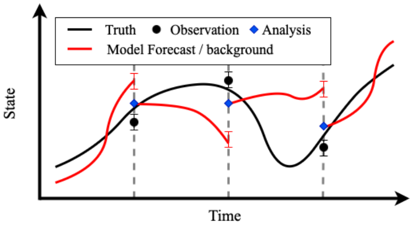
Earth system modeling presents a fundamental challenge in scientific computing: capturing complex, multiscale nonlinear dynamics in computationally efficient models while minimizing forecast errors caused by necessary simplifications. Even the most powerful AI- or physics-based forecast system suffer from gradual error accumulation. Data assimilation (DA) aims to mitigate these errors by optimally blending (noisy) observations with prior model forecasts, but conventional variational methods often assume Gaussian error statistics that fail to capture the true, non-Gaussian behavior of chaotic dynamical systems. We propose PnP-DA, a Plug-and-Play algorithm that alternates (1) a lightweight, gradient-based analysis update (using a Mahalanobis-distance misfit on new observations) with (2) a single forward pass through a pretrained generative prior conditioned on the background forecast via a conditional Wasserstein coupling. This strategy relaxes restrictive statistical assumptions and leverages rich historical data without requiring an explicit regularization functional, and it also avoids the need to backpropagate gradients through the complex neural network that encodes the prior during assimilation cycles. Experiments on standard chaotic testbeds demonstrate that this strategy consistently reduces forecast errors across a range of observation sparsities and noise levels, outperforming classical variational methods.
Figures


Figures from the paper (5 more)


Reference graph
Works this paper leans on
-
[1]
J. Amezcua, K. Ide, E. Kalnay, and S. Reich. Ensemble transform kalman–bucy filters. Quarterly Journal of the Royal Meteorological Society, 140(680):995–1004, 2014
work page 2014
-
[2]
D. Balwada, R. Abernathey, S. Acharya, A. Adcroft, J. Brener, V. Balaji, M. A. Bhouri, J. Bruna, M. Bushuk, W. Chapman, et al. Learning machine learning with lorenz-96. Journal of Open Source Education, 7(82):241, 2024
work page 2024
-
[3]
F. Bao, Z. Zhang, and G. Zhang. An ensemble score filter for tracking high-dimensional nonlinear dynamical systems.Computer Methods in Applied Mechanics and Engineering, 432:117447, 2024
work page 2024
-
[4]
K. Bi, L. Xie, H. Zhang, X. Chen, X. Gu, and Q. Tian. Accurate medium-range global weather forecasting with 3d neural networks.Nature, 619(7970):533–538, 2023
work page 2023
- [5]
- [6]
-
[7]
Carrassi, M
A. Carrassi, M. Bocquet, L. Bertino, and G. Evensen. Data assimilation in the geosciences: An overview of methods, issues, and perspectives.Wiley Interdisciplinary Reviews: Climate Change, 9(5):e535, 2018
2018
-
[8]
J. Chemseddine, P. Hagemann, G. Steidl, and C. Wald. Conditional wasserstein dis- tances with applications in bayesian ot flow matching.arXiv preprint arXiv:2403.18705, 2024. 17
arXiv 2024
Show all 57 references
-
[9]
Cheng, B
C. Cheng, B. Han, D. M. Robinson, A. F. Ansari, A. Stuart, M. Mahoney, and Y. B. Wang. Gradient-free generation for hard-constrained systems. 2025
2025
-
[10]
Cheng, C
S. Cheng, C. Quilodrán-Casas, S. Ouala, A. Farchi, C. Liu, P. Tandeo, R. Fablet, D. Lucor, B. Iooss, J. Brajard, et al. Machine learning with data assimilation and uncertainty quantification for dynamical systems: a review.IEEE/CAA Journal of Automatica Sinica, 10(6):1361–1387, 2023
2023
-
[11]
P. L. Combettes and J.-C. Pesquet. Proximal splitting methods in signal processing. Fixed-point algorithms for inverse problems in science and engineering, pages 185–212, 2011
2011
-
[12]
G. Evensen. The ensemble kalman filter for combined state and parameter estimation. IEEE Control Systems Magazine, 29(3):83–104, 2009
2009
-
[13]
Evensen, F
G. Evensen, F. C. Vossepoel, and P. J. Van Leeuwen. Iterative ensemble smoothers for data assimilation in coupled nonlinear multiscale models.Monthly Weather Review, 152(6):1277–1301, 2024
2024
-
[14]
H. Fan, B. Fei, P. Gentine, Y. Xiao, K. Chen, Y. Liu, Y. Qu, F. Ling, and L. Bai. Physically consistent global atmospheric data assimilation with machine learning in a latent space.arXiv preprint arXiv:2502.02884, 2025
2025
-
[15]
Farchi, M
A. Farchi, M. Chrust, M. Bocquet, P. Laloyaux, and M. Bonavita. Online model error correction with neural networks in the incremental 4d-var framework.Journal of Advances in Modeling Earth Systems, 15(9):e2022MS003474, 2023
2023
-
[16]
T. S. Finn, C. Durand, A. Farchi, M. Bocquet, P. Rampal, and A. Carrassi. Generative diffusion for regional surrogate models from sea-ice simulations.Journal of Advances in Modeling Earth Systems, 16(10):e2024MS004395, 2024
2024
-
[17]
Gaspari and S
G. Gaspari and S. E. Cohn. Construction of correlation functions in two and three dimensions. Quarterly Journal of the Royal Meteorological Society, 125(554):723–757, 1999
1999
-
[18]
Ghosh, V
S. Ghosh, V. Mons, D. Sipp, and P. J. Schmid. A robust computational framework for variational data assimilation of mean flows with sparse measurements corrupted by strong outliers. Journal of Computational Physics, 508:113008, 2024
2024
-
[19]
Huang, L
L. Huang, L. Gianinazzi, Y. Yu, P. D. Dueben, and T. Hoefler. Diffda: a diffusion model for weather-scale data assimilation.arXiv preprint arXiv:2401.05932, 2024
2024 arXiv
-
[20]
Kuramoto
Y. Kuramoto. Diffusion-induced chaos in reaction systems.Progress of Theoretical Physics Supplement, 64:346–367, 1978. 18
1978
-
[21]
K. J. Law, D. Sanz-Alonso, A. Shukla, and A. M. Stuart. Filter accuracy for the lorenz 96 model: Fixed versus adaptive observation operators.Physica D: Nonlinear Phenomena, 325:1–13, 2016
2016
-
[22]
S. Li, Y. Qu, T. Zheng, and P. Gentine. Machine-assisted physical closure for coarse suspended sediments in vegetated turbulent channel flows.Geophysical Research Letters, 51(20):e2024GL110475, 2024
2024
-
[23]
X. Liu, C. Gong, and Q. Liu. Flow straight and fast: Learning to generate and transfer data with rectified flow.arXiv preprint arXiv:2209.03003, 2022
2022 arXiv
-
[24]
E. N. Lorenz. Deterministic nonperiodic flow. Journal of Atmospheric Sciences, 20(2):130 – 141, 1963
1963
-
[25]
E. N. Lorenz. Predictability: A problem partly solved. InProc. Seminar on predictability, volume 1, pages 1–18. Reading, 1996
1996
-
[26]
Manshausen, Y
P. Manshausen, Y. Cohen, J. Pathak, M. Pritchard, P. Garg, M. Mardani, K. Kashinath, S. Byrne, and N. Brenowitz. Generative data assimilation of sparse weather station observations at kilometer scales.arXiv preprint arXiv:2406.16947, 2024
2024 arXiv
-
[27]
Mardani, J
M. Mardani, J. Song, J. Kautz, and A. Vahdat. A variational perspective on solving inverse problems with diffusion models.arXiv preprint arXiv:2305.04391, 2023
2023 arXiv
-
[28]
Martin, A
S. Martin, A. Gagneux, P. Hagemann, and G. Steidl. Pnp-flow: Plug-and-play image restoration with flow matching.arXiv preprint arXiv:2410.02423, 2024
2024 arXiv
-
[29]
Palmer and B
T. Palmer and B. Stevens. The scientific challenge of understanding and estimating climate change.Proceedings of the National Academy of Sciences, 116(49):24390–24395, 2019
2019
-
[30]
T. N. Palmer. A nonlinear dynamical perspective on model error: A proposal for non-local stochastic-dynamic parametrization in weather and climate prediction models. Quarterly Journal of the Royal Meteorological Society, 127(572):279–304, 2001
2001
-
[31]
Pasmans, Y
I. Pasmans, Y. Chen, T. S. Finn, M. Bocquet, and A. Carrassi. Ensemble kalman filter in latent space using a variational autoencoder pair.arXiv preprint arXiv:2502.12987, 2025
2025 arXiv
-
[32]
Price, A
I. Price, A. Sanchez-Gonzalez, F. Alet, T. R. Andersson, A. El-Kadi, D. Masters, T. Ewalds, J. Stott, S. Mohamed, P. Battaglia, et al. Probabilistic weather forecasting with machine learning.Nature, 637(8044):84–90, 2025
2025
-
[33]
Protas, T
B. Protas, T. R. Bewley, and G. Hagen. A computational framework for the regulariza- tion of adjoint analysis in multiscale pde systems.Journal of Computational Physics, 195(1):49–89, 2004. 19
2004
-
[34]
Y. Qu, M. A. Bhouri, and P. Gentine. Joint parameter and parameterization inference with uncertainty quantification through differentiable programming.arXiv preprint arXiv:2403.02215, 2024
2024 arXiv
-
[35]
Y. Qu, J. Nathaniel, S. Li, and P. Gentine. Deep generative data assimilation in multimodal setting. InProceedings of the IEEE/CVF Conference on Computer Vision and Pattern Recognition, pages 449–459, 2024
2024
-
[36]
Qu and X
Y. Qu and X. Shi. Can a machine learning–enabled numerical model help extend effective forecast range through consistently trained subgrid-scale models?Artificial Intelligence for the Earth Systems, 2(1):e220050, 2023
2023
-
[37]
V. Rao, A. Sandu, M. Ng, and E. D. Nino-Ruiz. Robust data assimilation using l_1 and huber norms.SIAM Journal on Scientific Computing, 39(3):B548–B570, 2017
2017
-
[38]
Ruckstuhl, T
Y. Ruckstuhl, T. Janjić, and S. Rasp. Training a convolutional neural network to conserve mass in data assimilation.Nonlinear Processes in Geophysics, 28(1):111–119, 2021
2021
-
[39]
E. Ryu, J. Liu, S. Wang, X. Chen, Z. Wang, and W. Yin. Plug-and-play methods provably converge with properly trained denoisers. InInternational Conference on Machine Learning, pages 5546–5557. PMLR, 2019
2019
-
[40]
Sivashinsky
G. Sivashinsky. Nonlinear analysis of hydrodynamic instability in laminar flames—i. derivation of basic equations. In P. Pelcé, editor,Dynamics of Curved Fronts, pages 459–488. Academic Press, San Diego, 1988
1988
-
[41]
Solvik, S
K. Solvik, S. G. Penny, and S. Hoyer. 4d-var using hessian approximation and back- propagation applied to automatically-differentiable numerical and machine learning models. arXiv preprint arXiv:2408.02767, 2024
2024 arXiv
-
[42]
S. K. Tamang, A. Ebtehaj, P. J. Van Leeuwen, D. Zou, and G. Lerman. Ensemble riemannian data assimilation over the wasserstein space. Nonlinear Processes in Geophysics Discussions, 2021:1–26, 2021
2021
-
[43]
S. V. Venkatakrishnan, C. A. Bouman, and B. Wohlberg. Plug-and-play priors for model based reconstruction. In2013 IEEE global conference on signal and information processing, pages 945–948. IEEE, 2013
2013
-
[44]
Z. Wu, Y. Sun, Y. Chen, B. Zhang, Y. Yue, and K. Bouman. Principled probabilistic imaging using diffusion models as plug-and-play priors.Advances in Neural Information Processing Systems, 37:118389–118427, 2024
2024
-
[45]
Y. Xiao, Q. Jia, W. Xue, and L. Bai. Vae-var: Variational-autoencoder-enhanced variational assimilation.arXiv preprint arXiv:2405.13711, 2024. 20
2024 arXiv
-
[46]
X. Xu, X. Sun, W. Han, X. Zhong, L. Chen, Z. Gao, and H. Li. Fuxi-da: A generalized deep learning data assimilation framework for assimilating satellite observations.npj Climate and Atmospheric Science, 8(1):156, 2025
2025
-
[47]
X. Zhu, Y. Qu, and X. Shi. Lex v1.4: A new large-eddy simulation model in jax with gpu acceleration and automatic differentiation.EGUsphere, 2025:1–26, 2025
2025
-
[48]
Y. Zhu, K. Zhang, J. Liang, J. Cao, B. Wen, R. Timofte, and L. Van Gool. Denoising diffusion models for plug-and-play image restoration. InProceedings of the IEEE/CVF Conference on Computer Vision and Pattern Recognition, pages 1219–1229, 2023. A Experimental Setup Lorenz-63 D...
2023
-
[49]
• Use 4th-order Runge–Kutta (RK4) with step size∆t = 0.01
Nature Run: • Integrate the true Lorenz-63 system dx dt = −σ (x − y), dy dt = ρ x− y − x z, dz dt = x y− β z, with parameters σ = 10, ρ= 28, β = 8/3. • Use 4th-order Runge–Kutta (RK4) with step size∆t = 0.01. • Spin-up for 5000 steps, discard first 1000 • Record trajectory xt ...
-
[50]
• Generate noisy observations yk = xtk + εk, ε k ∼ N(0, Σobs), with Σobs = σ2 obs C, σobs = √ 2, and C = 1 0 .5 0 .25 0.5 1 0 .5 0.25 0 .5 1
Synthetic Observations: • Observation times tk = k × 40 ∆t (every 40 steps,∆tobs = 0.4). • Generate noisy observations yk = xtk + εk, ε k ∼ N(0, Σobs), with Σobs = σ2 obs C, σobs = √ 2, and C = 1 0 .5 0 .25 0.5 1 0 .5 0.25 0 .5 1
-
[51]
Initialize x(i) 0 = x0 + δ(i), δ (i) ∼ N(0, σ2 initI3), σinit = √ 2
Ensemble Riemannian DA (EnRDA) Loop: [42] • Ensemble size N = 10. Initialize x(i) 0 = x0 + δ(i), δ (i) ∼ N(0, σ2 initI3), σinit = √ 2. 21 • Forecast step: each member is propagated under a perturbedoperational model with parameters (σ′, ρ′, β′) = (10.5, 27.0, 10/3) via xb,(i) ...
-
[52]
• Use 4th-order Runge–Kutta with∆t = 0.005; spin-up 10,000 steps, discard first 2,000
Nature Run: • Integrate the two-scale Lorenz-96 system dXk dt = −Xk−1 (Xk−2 − Xk+1) − Xk + F + h c b JX j=1 Yj,k, dYj,k dt = −c b Yj+1,k (Yj+2,k − Yj−1,k) − c Yj,k + h c b Xk, with K = 8, J = 32, F = 18, h = 1, b = c = 10. • Use 4th-order Runge–Kutta with∆t = 0.005; spin-up 10...
-
[53]
• Corrupt with Gaussian noise yk = Xk(tk) + εk, ε k ∼ N(0, σ2 obs), σobs = 0.5
Synthetic Observations: • Observe 50% of slow variablesXk every ∆tobs = 0.2. • Corrupt with Gaussian noise yk = Xk(tk) + εk, ε k ∼ N(0, σ2 obs), σobs = 0.5. 22
-
[54]
• Analysis: – Computebackgroundmean ¯xb andcovariance B = 1 N −1 P i(xb,(i)−¯xb)(xb,(i)− ¯xb)⊤
Cyclic EnKF Assimilation (N=20): • Forecast: Propagate each analysis memberxa,(i) tk−1 under the single-scale Lorenz-96 model dXk dt = −Xk−1 (Xk−2 − Xk+1) − Xk + F ′, with F ′ = 18, over ∆tobs to obtain background ensemble{xb,(i) tk }. • Analysis: – Computebackgroundmean ¯xb a...
-
[55]
• Discretize into ne = 128 interior points; use LSODA solver with∆t = 0.25
Nature Run: • Integrate the Kuramoto–Sivashinsky equation ∂u ∂t = −u ∂u ∂x − ∂2u ∂x2 − ν ∂4u ∂x4 , on x ∈ [0, L] with Dirichlet BCsu(0) = u(L) = 0, where ν = 0.5, L = 50. • Discretize into ne = 128 interior points; use LSODA solver with∆t = 0.25. • Spin-up for tini = 50 (ns=20...
-
[56]
• Add independent noise uobs = utrue(xobs, tb) + ε, ε ∼ N(0, σ2 obs), σobs = √ 10−2
Synthetic Observations: • Observe me = 16 equally spaced grid points at timestb = k (tmax/nf ), where nf = 10. • Add independent noise uobs = utrue(xobs, tb) + ε, ε ∼ N(0, σ2 obs), σobs = √ 10−2
-
[57]
• Analysis: At each tb: – Perturb observations: uo,(i) = uobs + δ(i), δ(i) ∼ N(0, σ2 obsI)
Cyclic EnKF Assimilation (N=40): 23 • Forecast: For each ofN = 40 members, integrate the “bad” forecast model (same KS but adding process noise) ub,(i) t+∆t = LSODA ua,(i) t + η, η ∼ N(0, σ2 modI), σmod = √ 10−2. • Analysis: At each tb: – Perturb observations: uo,(i) = uobs + ...
Reviewed August 6, 2026 · model on record in the stance chip above.
Discussion (0). Sign in to comment.