Critical fluid dynamics in two and three dimensions

Chandrodoy Chattopadhyay; Josh Ott; Thomas Schaefer; Vladimir V. Skokov

REVIEW 3 major objections 4 minor 3 cited by

Critical fluid dynamics in two and three dimensions

T0 review · 3 major / 4 minor · reviewed 2026-08-12 · deepseek-v4-flash

Challenge this review Re-run · record.json Download PDF Read on arXiv ↗ Review JSON

Pith's one-line read The Metropolis lattice algorithm simulates stochastic fluid dynamics near a critical point and measures the dynamic critical exponent $z\simeq3$ in three dimensions and $z\simeq2$ in two dimensions.

desk verdict Solid 3D model H result, but the new 2D claim rests on an untested truncation and a thin finite-size extraction. read the letter →

arxiv 2411.15994 v2 pith:U56PIJBY submitted 2024-11-24 nucl-th hep-lathep-ph

Chandrodoy Chattopadhyay , Josh Ott , Thomas Schaefer , Vladimir V. Skokov This is my paper · ORCID

classification nucl-thhep-lathep-ph

keywords stochasticfluiddynamicsmodelHdynamiccriticalexponentMetropolisalgorithmpointIsinguniversalityclassQCDendpointfinite-sizescaling

verification ladder T0 review T1 audit T2 compute T3 formal

The pith

A machine-rendered reading of the paper's core claim, the machinery that carries it, and where it could break.

The reading

This paper introduces a Metropolis accept-reject update for stochastic fluid dynamics in the Ising universality class, the theory known as model H, and uses it to measure the dynamic critical exponent $z$. Because the same step produces both diffusion and thermal noise, fluctuation-dissipation balance is automatic and the equilibrium distribution is governed solely by the microscopic free energy. In three dimensions the authors report $z\simeq3$, with a best value $z_{\rm eff}=3.013\pm0.058$, and in two dimensions they find $z\simeq2$, with a measured value $2.11\pm0.015$ at the smallest viscosity simulated. They also observe a finite-size crossover from the mean-field value $z=4$ to the critical value, controlled by the correlation length and the renormalized shear viscosity. This matters because model H is expected to describe the non-equilibrium dynamics of the quark-gluon plasma near a possible critical endpoint, where existing analytic methods are low-order and hard to extend to expanding flows.

What carries the argument

The object that carries the argument is a local, conserving Metropolis update: a random amount of the conserved field, either $\phi$ or the momentum density, is moved between neighboring lattice sites and the move is accepted with probability $\min(1,e^{-\Delta H/T})$. The first moment of this step reproduces the dissipative current and the second moment supplies the noise, so fluctuation-dissipation balance is automatic and equilibrium is governed by the Hamiltonian alone. The advective mode-coupling terms are integrated with a strong-stability-preserving Runge-Kutta scheme and a skew-symmetric spatial discretization that conserves kinetic energy, and after each sweep the momentum field is projected onto transverse modes in Fourier space. The diagnostic that fixes $z$ is the dynamic scaling collapse of the order-parameter correlation function, $C_\phi(t,k;L)=\tilde C_\phi(t/L^z,kL)$, compared between two volumes.

What would settle it

Run full model H, with the self-advection term included, in two dimensions at bare viscosity $\eta=10^{-2}$ on $L=40$ and $L=48$ lattices, and check whether the order-parameter correlation functions collapse with $z\approx2$; if a clearly different exponent is required, the reported two-dimensional asymptotic value is not the exponent of the full model H.

Watch

Extended reading notes

Core claim

The central claim is that the Metropolis algorithm correctly simulates model H and that the dynamic critical exponent takes its standard values: $z\simeq3$ in three dimensions and $z\simeq2$ in two dimensions. The best three-dimensional estimate, $z_{\rm eff}=3.013\pm0.058$ at renormalized viscosity $\eta_R=10^{-2}$, is obtained by demanding data collapse of the order-parameter correlation function $C_\phi(t,k;L)$ under the rescaling $t\to(40/48)^z t$ for lattices with $L=40$ and $L=48$. In two dimensions the measured value at bare viscosity $\eta=10^{-2}$ is $z=2.11\pm0.015$, and the paper argues that the asymptotic value is $z\simeq2$. The two-dimensional extraction is performed in model H0, the truncation of model H without the self-advection of the transverse momentum, which the authors expect to lie in the same dynamical universality class as model H. A crossover from the mean-field value $z=4$ to the critical value is observed and is semi-quantitatively described by the mode-coupling relaxation-rate formula used in the paper, with the crossover governed by the correlation length and the renormalized shear viscosity.

Load-bearing premise

The two-dimensional result is extracted from model H0, a truncation that drops the self-advection of the transverse momentum, and the analysis assumes both that model H0 lies in the same dynamical universality class as model H and that two volumes and one momentum mode are enough to determine the infinite-volume exponent.

Editorial extensions

If this is right

The measured $z\simeq3$ in $d=3$ agrees with two-loop epsilon-expansion values and provides direct numerical confirmation of model-H dynamic scaling.
The observed crossover from $z=4$ to the critical exponent means finite systems will generically show effective exponents between these limits, so size and viscosity must be controlled before comparing to experiments.
Because equilibrium is independent of the transport coefficients, the same Metropolis update can be reused at different viscosities and densities without re-tuning the noise.
The two-dimensional measurement gives $z\simeq2.11\pm0.015$ at the smallest viscosity simulated, with asymptotic $z\simeq2$, supplying a numerical reference in a dimension where analytic methods are least controlled.

Reading between the lines

Editorial extensions of the paper, not claims the author makes directly.

If the model-H0 and model-H universality assumption holds, the two-dimensional result is a first direct numerical value for the $d=2$ critical fluid; simulating the full two-dimensional model H at the same parameters would test this identification.
The paper's own estimate that the critical enhancement of $\eta_R$ between $L=40$ and $L=48$ is only about one percent suggests that isolating the universal part of the shear viscosity will require substantially larger volumes or a different estimator.
The Metropolis framework is naturally suited to non-equilibrium and expanding flows, so the main obstacle to QCD-relevant simulations is likely to be the renormalization of the equation of state rather than the noise implementation.

Share X Bluesky LinkedIn Reddit HN

Editorial analysis

A structured set of objections, weighed in public.

Desk editor's note, referee report, and a circularity audit.

Desk Editor's Note

read the letter

First thing to know: this is the detailed companion to the model H PRL, and most of the value is in the method rather than a new exponent. The 3D result z = 3.013 ± 0.058 at ηR = 10^-2 is consistent with the epsilon expansion and with the companion PRL; that is a genuine confirmation. What is actually new in this manuscript is the lattice implementation of the Metropolis update with skew-symmetric advection, the viscosity renormalization study (Fig. 7), and the first 2D dynamic scaling result.

The algorithm deserves credit. The skew-symmetric discretization preserves energy conservation for the advection steps, the checkerboard Metropolis update is local and conserving, and the code and data are deposited. Static tests pass, though they are partly self-consistency checks because the Metropolis step enforces the equilibrium distribution. The dynamic exponent extraction is a measurement, not an input, and the crossover from z = 4 to z = 3 as a function of ηR is well presented and semi-quantitatively matches Kawasaki.

Now the soft spots. The 2D claim z ≈ 2 is extracted exclusively from model H0, the truncation that drops the π^T self-advection. The paper justifies this by the relative damping rates, but in d = 2 that argument is marginal: at z = 2 the ratio (Γk^4)/( (η/ρ)k^2 ) behaves as k^0, so the two mode-couplings are marginal relative to each other at the fixed point. The stress-test note has this right. The authors do not simulate full model H in 2D, and the existing 2D viscosity literature already has log divergences. So the reported 2D exponent may be the exponent of a different theory. At minimum the claim should be softened to “model H0 in 2D” and the truncation tested, for example by running full model H at one small η.

Second, the finite-size extraction is thin. Two volumes, one momentum mode, and a window C(t) > 0.15. The quoted statistical error, z = 2.11 ± 0.015, is suspiciously small given that the two-volume collapse has no systematic scan over modes or fitting windows. Missing error bars in several key figures make it hard to judge the scatter. This is more a presentation and robustness issue than a fatal flaw.

Third, trivial but embarrassing: refs [78] and [79] give the same Zenodo DOI. That should be corrected.

Who is this for? People building stochastic hydrodynamic simulations for the QCD critical endpoint, and anyone interested in nonperturbative methods for critical dynamics. It deserves serious refereeing; the 3D part is solid, and the 2D result is worth publishing after the truncation concern is addressed head-on. I would accept for review with the expectation of a major revision on the 2D section.

Referee Report

3 major / 4 minor

Summary. The manuscript develops a Metropolis-based lattice algorithm for stochastic model H hydrodynamics, in which the dissipative update and noise are combined so that the equilibrium distribution is the Gibbs distribution of the microscopic Hamiltonian. The method is applied to a conserved Ising-type order parameter coupled to transverse momentum density in d=3 and d=2. Static checks (magnetization histograms, subvolume scaling, correlation functions) are presented, the momentum correlation function is used to extract a renormalized shear viscosity, and the order-parameter correlation function is used to extract effective dynamic critical exponents via finite-size dynamic scaling with L=40 and L=48. In three dimensions the authors report z_eff=3.013±0.058 at ηR=10^-2, with a crossover from z≈4 to z≈3 that they compare with the Kawasaki approximation. In two dimensions, using only model H0 (model H without the transverse momentum self-advection), they report z=2.11±0.015 at η=10^-2 and argue for an asymptotic value z≈2.

Significance. If the central claims hold, the paper provides a direct numerical test of model H dynamic scaling and demonstrates a practical method for stochastic fluid dynamics near a critical point, which is relevant for QCD critical-endpoint phenomenology. The Metropolis construction is attractive because fluctuation-dissipation relations are satisfied by construction, the static equilibrium behavior can be checked directly, and the code is deposited on Zenodo, which is a concrete reproducibility asset. The three-dimensional result, including the agreement between model H and model H0 when plotted against the renormalized viscosity, is a genuine measurement rather than an input. However, the two-dimensional conclusion is substantially weaker: it rests entirely on model H0, a universality assumption that is not verified in d=2, and on a two-volume, one-mode finite-size scaling analysis. Because the 2D claim appears in the abstract as a headline result, this limitation is load-bearing.

major comments (3)

[§V.D, Fig. 11] The two-dimensional dynamic exponent is extracted exclusively from model H0, not from the full model H. The justification in §II.B that the π^T self-advection can be neglected relies on the disparity between shear damping (η/ρ)k^2 and order-parameter damping Γk^4; at z≈2 in d=2 that ratio behaves as k^{z-2}=k^0, so the two mode-coupling terms are marginal relative to each other and the truncation is not obviously innocuous. Since §V.D states that the renormalized viscosity was not studied in 2D and no full model H simulation is reported, the quoted z≈2 is presently a measurement of model H0 rather than of model H. The claim should be supported by a 2D model H run or explicitly qualified as a model H0 result with an assessment of the universality risk.
[§V.C–V.D, Figs. 8, 9, 11] The quoted exponents are derived from a single pair of volumes (L=40 and L=48), the second non-trivial momentum mode, and the collapse window C(t)>0.15, with no documented scan over the fitting window, the momentum mode, or additional lattice sizes. The statistical errors (for example z=2.11±0.015 in 2D) therefore do not include finite-size scaling or analysis-parameter systematics, and the extrapolation from z=2.11 to the asymptotic value z≈2 is made without an estimate of those systematics. The authors should report stability of the extracted exponents under variation of the window, mode number, and volume range, or state a corresponding systematic uncertainty.
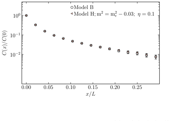
[§V.A] The manuscript itself notes a shift in the critical bare mass for model H, δm2_c=-0.03 in 3D, attributed to the advection step not exactly conserving the potential-energy part of the Hamiltonian. This means the discretized dynamics does not sample exactly the target Hamiltonian, and the shift must be determined empirically. The text does not state explicitly which critical mass value is used in the 2D dynamic scaling runs (the model A/B value m2_c=-3.8240±0.0003 or the shifted model H value m2_c≈-3.859), and the uncertainty in this empirical shift is not propagated into the extracted exponent. Please state the value used and estimate the resulting systematic uncertainty.

minor comments (4)

[Footnote 80] There is a typo: 'centererd derivative kinetic energy' should read 'centered derivative kinetic energy'.
[References [78,79]] References [78] and [79] list the same Zenodo DOI (10.5281/zenodo.14706997); if the 2D and 3D data sets have separate DOIs, the second DOI should be corrected.
[Fig. 7] The caption states that self-advection results are offset horizontally for readability, but the offset is not quantified; adding the offset value to the caption would make the figure self-contained.
[Eq. (67) and Fig. 9] The Kawasaki comparison uses only the broad estimate ξ∈[L/(2π),L/2] for the finite-volume correlation length; this yields a wide band and makes the comparison semi-quantitative. A direct measurement of the finite-volume correlation length from the static correlator would strengthen the crossover test.

Circularity Check

0 steps flagged · score 0.0 of 10

No significant circularity: the dynamic exponent is measured via finite-size collapse, and the 2D H0 truncation is an unverified universality assumption rather than a circular reduction.

full rationale

The paper's central quantities, z in d=3 and d=2, are extracted by a direct finite-size scaling procedure: the correlation function C(t,k;L) is computed at two volumes (L=40,48) and a scaling exponent z is obtained by requiring collapse of C(alpha t, kL) with alpha=(40/48)^z (Figs. 8 and 11). This is a measurement, not an output of the theory being tested. The comparison with the Kawasaki approximation (Eq. (67)) uses the renormalized shear viscosity measured independently from the momentum-density correlation function (Eq. (62), Fig. 6) and a stated range xi in [L/2pi, L/2], so it is not a fit that forces the measured z. The Metropolis update is constructed by detailed balance to sample exp(-H/T), so the static distribution checks in Section V.A are self-consistency validations of the algorithm rather than independent predictions; the paper does not present them as the derivation of z. The critical point m_c^2 is an input taken from the authors' prior Binder-cumulant studies, but it is not the target result and is anchored to known universal values, so this self-citation is not load-bearing for the dynamic exponent. The most substantive weakness is the two-dimensional claim: z≈2 is obtained from model H0, not full model H, based on the expectation of the same dynamical universality class. That is an unverified physical assumption about external validity, not a circularity in which the output is equivalent to an input by construction. No equation in the paper reduces z to the model parameters or to the self-citations invoked.

Assumptions & free parameters 5 free parameters · 6 assumptions · 0 invented entities

The central measurement rests on the standard model H Lagrangian, a critical-mass tuning from the authors' previous Binder analyses, and a Metropolis scheme whose equilibrium distribution is enforced by construction. The main fitted inputs are m_c^2, ηR, and the model H critical shift; universality assumptions about the truncation and finite-size scaling carry the 2D claim.

free parameters (5)

Critical bare mass m_c^2 (3D) = -2.28587(7) in model A; model H uses m_c^2 - 0.03
Determined from Binder cumulant crossings in the authors' earlier model A work; used to set the simulation at the critical point where the dynamic exponent is extracted. The model H shift is calibrated against the model B static correlator.
Critical bare mass m_c^2 (2D) = -3.8240(3) in model A; model H uses -3.859
Determined from Binder cumulant crossings and a finite-size fit; needed for the 2D dynamic scaling measurement.
Bare shear viscosity η = 10^-2 to 10^2 (3D); 10^-3 to 10^1 (2D)
Control parameter of model H. The dynamic exponent is extracted at small η, where shear damping is weak; results are plotted against η and against the renormalized ηR.
Renormalized shear viscosity ηR = approximately 0.3 for model H at η = 0.01, ρ = 1; approximately 10^-2 for model H0
Extracted by fitting the plateau in k^-2 d ln Cπ(t)/dt (Fig. 6). Used as the physical viscosity in the Kawasaki crossover comparison, so that comparison is not fully parameter-free.
Scalar self-coupling λ = λ = 4
Chosen by hand; universality makes the critical dynamics independent of its value, but it sets the lattice action used in the simulations.

assumptions (6)

domain assumption Model H equations (1)-(6) correctly describe the long-wavelength critical dynamics of a fluid in the Ising universality class, including the QCD critical endpoint.
Taken from the Hohenberg-Halperin classification and the QCD critical endpoint literature (refs 12-14); not derived in this paper.
domain assumption The Metropolis update with Gaussian trial moves of variance 2ΓTΔt and acceptance probability min(1, e^{-ΔH/T}) converges to the model H Langevin dynamics in the small timestep limit.
Core algorithmic assumption; supported by static equilibrium checks and previous model A/B papers, but no convergence proof is given here. The mathematical reference [50] is cited for the general scheme.
domain assumption The dynamic scaling relation Cϕ(t, k; L) = C̃ϕ(t/L^z, kL) holds for the simulated finite systems.
Standard hypothesis used to extract z from two volumes and one momentum mode; not independently verified over more system sizes.
domain assumption Model H0, which drops the self-advection of πT, lies in the same dynamical universality class as model H.
Authors state this expectation in Section II.B and use model H0 for the 2D measurement; no direct 2D full-model-H check is provided.
ad hoc to paper The Kawasaki approximation Eq. (67), with renormalized ηR and a correlation length bounded between L/(2π) and L/2, describes the observed crossover.
Used to produce the crossover band in Fig. 9; requires in-sample ηR and a loose ξ range, so the comparison is semi-quantitative.
domain assumption The transverse projection after each update step preserves the equilibrium Gibbs distribution and correctly implements the constraint ∇·πT = 0.
Numerical construction; the authors verify the static distribution of ϕ and the equidistribution of πT, but do not prove that the projection preserves detailed balance.

how reviews work

0 comments

Cite this review

Pith. "Pith review of Critical fluid dynamics in two and three dimensions." pith.science (2026). https://pith.science/paper/U56PIJBY

@misc{pith2026241115994,
  author       = {Pith},
  title        = {Pith review of: Critical fluid dynamics in two and three dimensions},
  year         = {2026},
  howpublished = {\url{https://pith.science/paper/U56PIJBY}},
  note         = {Machine review of arXiv:2411.15994}
}

abstract

We describe a numerical method for simulating stochastic fluid dynamics near a critical point in the Ising universality class. This theory is known as model H, and is expected to govern the non-equilibrium dynamics of Quantum Chromodynamics (QCD) near a possible critical endpoint of the phase transition between a hadron liquid and the quark-gluon plasma. The numerical algorithm is based on a Metropolis scheme, and automatically ensures that the distribution function of the hydrodynamic variables in equilibrium is independent of the transport coefficients and only governed by the microscopic free energy. We verify dynamic scaling near the critical point of a two and three-dimensional fluid and extract the associated critical exponent $z$. We find $z\simeq 3$ in three dimensions, and $z\simeq 2$ for a two-dimensional fluid. In a finite system, we observe a crossover between the mean field value $z=4$ and the true critical exponent $z\simeq 3$ ($z \simeq 2$ in $d=2$). This crossover is governed by the values of the correlation length and the renormalized shear viscosity.

Figures

Figures reproduced from arXiv: 2411.15994 by the authors.

**Figure 2.** FIG. 2: Three-dimensional renderings of the order parameter [PITH_FULL_IMAGE:figures/full_fig_p020_2.png] view at source ↗

**Figure 3.** FIG. 3: The left panel shows the histogram of the magnetization [PITH_FULL_IMAGE:figures/full_fig_p021_3.png] view at source ↗

Figures from the paper (8 more)

**Figure 4.** Figure 4: FIG. 4: The left panel shows the histogram of sub-volume magnetization [PITH_FULL_IMAGE:figures/full_fig_p022_4.png]

**Figure 5.** Figure 5: FIG. 5: Static correlation function of the order parameter [PITH_FULL_IMAGE:figures/full_fig_p023_5.png]

**Figure 6.** Figure 6: FIG. 6: Logarithmic derivative [PITH_FULL_IMAGE:figures/full_fig_p024_6.png]

**Figure 7.** Figure 7: FIG. 7: Physical viscosity as a function of the bare viscosity in four different theories: 1) Model [PITH_FULL_IMAGE:figures/full_fig_p025_7.png]

**Figure 8.** Figure 8: FIG. 8: Normalized dynamic order parameter correlation function [PITH_FULL_IMAGE:figures/full_fig_p027_8.png]

**Figure 9.** Figure 9: FIG. 9: Left panel: Dynamic scaling exponent [PITH_FULL_IMAGE:figures/full_fig_p028_9.png]

**Figure 10.** Figure 10: FIG. 10: Left panel: Binder cumulant for model A in two dimensions as a function of the control [PITH_FULL_IMAGE:figures/full_fig_p029_10.png]

**Figure 11.** Figure 11: FIG. 11: Left panel: Dynamic scaling of the normalized order parameter correlation function [PITH_FULL_IMAGE:figures/full_fig_p030_11.png]

Discussion (0). Continue with ORCID to comment.

Forward citations

Cited by 3 Pith papers

Reviewed papers in the Pith corpus that reference this work. Sorted by Pith novelty score. Full citation record

Initial-State Charge Density Predicts Final-State Net Charge Flow in Heavy-Ion Collisions
nucl-th 2025-05 conditional novelty 6.0 of 10

Initial baryon density, through a charge-odd cumulant estimator with a fitted coupling, predicts final net-proton elliptic flow in event-by-event hydrodynamic simulations.
Simulating stochastic fluid dynamics
nucl-th 2025-08 conditional novelty 3.0 of 10

First simulations of model H stochastic fluid dynamics near a critical point give a dynamic critical exponent z ≈ 3.01 and viscosity renormalization.
Theory Summary
nucl-th 2025-09 unverdicted

A conference summary paper reports selected theory results from Quark Matter 2025 in heavy-ion physics, with no new original research.

Reference graph

Works this paper leans on

89 extracted references · 35 canonical work pages · cited by 3 Pith papers

[78]

Ohta, Progress of Theoretical Physics 54, 1566 (1975)

T. Ohta, Progress of Theoretical Physics 54, 1566 (1975)

work page 1975
[79]

L. P. Kadanoff, G. R. McNamara, and G. Zanetti, Phys. Rev. A 40, 4527 (1989)

work page 1989
[1]

Model H as defined by Eqs. (1,2). The discretized form of the advection terms is given in Eqs. (41,42), and the dissipative terms are defined in Eqs. (47-52). 23 0 20 40 60 80 100 0.1 0.2 0.3 0.4 0.5 0.6 t 1 k2 d dt ln(Cπ(t, k)) η = 0.01 η = 0.05 FIG. 6: Logarithmic derivative k−2d log Cπ(t)/dt of the two-point function of the momentum den- sity Cπ(t, ⃗k)...
[2]

(2) and (42)

Model H0, which we have defined as Model H without the self-advection term in Eqs. (2) and (42). As discussed in Sect. II B, model H0 is a consistent truncation of model H which is expected to be in the same dynamical universality class
[3]

(1,2) and Eqs

Pure self advection, which takes into account the non-linear dynamics of the momen- tum density, but ignores the coupling between ϕ and ⃗ πT in Eqs. (1,2) and Eqs. (41,42). In this theory the momentum density is decoupled from the critical dynamics of the order parameter
[4]

In this approximation, the equation of the momentum density is completely linear

Pure momentum diffusion, which corresponds to ignoring all mode couplings. In this approximation, the equation of the momentum density is completely linear. The last of these theories, pure momentum diffusion, only serves as a very basic check of our numerical procedure. Indeed, the open circles in Fig. 7 show that the physical viscosity is very close to ...
[5]

Kovtun, G

P. Kovtun, G. D. Moore, and P. Romatschke, Phys. Rev. D 84, 025006 (2011), arXiv:1104.1586 [hep-ph]

arXiv 2011
[6]

Sch¨ afer and D

T. Sch¨ afer and D. Teaney, Rept. Prog. Phys.72, 126001 (2009), arXiv:0904.3107 [hep-ph]

arXiv 2009

Show all 89 references

[7]

Jeon and U

S. Jeon and U. Heinz, Int. J. Mod. Phys. E 24, 1530010 (2015), arXiv:1503.03931 [hep-ph]

2015 arXiv
[8]

Romatschke and U

P. Romatschke and U. Romatschke, Relativistic Fluid Dynamics In and Out of Equilib- rium, Cambridge Monographs on Mathematical Physics (Cambridge University Press, 2019) arXiv:1712.05815 [nucl-th]

2019 arXiv
[9]

Landau and E

L. Landau and E. Lifshitz, Course of Theoretical Physics: Statistical Physics,Part 2(Perga- mon Press, 1980)

1980
[10]

Chao and T

J. Chao and T. Sch¨ afer, JHEP01, 071 (2021), arXiv:2008.01269 [hep-th]

2021 arXiv
[11]

Crossley, P

M. Crossley, P. Glorioso, and H. Liu, JHEP 09, 095 (2017), arXiv:1511.03646 [hep-th]

2017 arXiv
[12]

Chen-Lin, L

X. Chen-Lin, L. V. Delacr´ etaz, and S. A. Hartnoll, Phys. Rev. Lett. 122, 091602 (2019), arXiv:1811.12540 [hep-th]

2019 arXiv
[13]

Jain and P

A. Jain and P. Kovtun, Phys. Rev. Lett. 128, 071601 (2022), arXiv:2009.01356 [hep-th]

2022 arXiv
[14]

L. V. Delacretaz, SciPost Phys. 9, 034 (2020), arXiv:2006.01139 [hep-th]

2020 arXiv
[15]

Arcovito, C

G. Arcovito, C. Faloci, M. Roberti, and L. Mistura, Phys. Rev. Lett. 22, 1040 (1969)

1969
[16]

Basar, (2024), arXiv:2410.02866 [hep-th]

G. Basar, (2024), arXiv:2410.02866 [hep-th]

2024 arXiv
[17]

P. C. Hohenberg and B. I. Halperin, Rev. Mod. Phys. 49, 435 (1977)

1977
[18]

Rajagopal and F

K. Rajagopal and F. Wilczek, Nucl. Phys. B 399, 395 (1993), arXiv:hep-ph/9210253

1993 arXiv
[19]

D. T. Son and M. A. Stephanov, Phys. Rev. D 70, 056001 (2004), arXiv:hep-ph/0401052

2004 arXiv
[20]

J. V. Roth and L. von Smekal, JHEP 10, 065 (2023), arXiv:2303.11817 [hep-ph]

2023 arXiv
[21]

Canet and H

L. Canet and H. Chate, J. Phys. 40, 1937 (2007), arXiv:cond-mat/0610468

2007 arXiv
[22]

Canet, H

L. Canet, H. Chate, and B. Delamotte, J. Phys. A 44, 495001 (2011), arXiv:1106.4129 [cond- mat.stat-mech]

2011 arXiv
[23]

Mesterh´ azy, J

D. Mesterh´ azy, J. H. Stockemer, L. F. Palhares, and J. Berges, Phys. Rev. B 88, 174301 (2013), arXiv:1307.1700 [cond-mat.stat-mech]

2013 arXiv
[24]

Chen, Y.-y

Y.-r. Chen, Y.-y. Tan, and W.-j. Fu, Phys. Rev. D 109, 094044 (2024), arXiv:2312.05870 [hep-ph] . 32

2024 arXiv
[25]

Akamatsu, A

Y. Akamatsu, A. Mazeliauskas, and D. Teaney, Phys. Rev. C 95, 014909 (2017), arXiv:1606.07742 [nucl-th]

2017 arXiv
[26]

Chen, Y.-Y

Y.-R. Chen, Y.-Y. Tan, and W.-J. Fu, (2024), arXiv:2406.00679 [hep-ph]

2024 arXiv
[27]

J. V. Roth, Y. Ye, S. Schlichting, and L. von Smekal, (2024), arXiv:2409.14470 [hep-ph]

2024 arXiv
[28]

J. I. Kapusta, B. Muller, and M. Stephanov, Phys. Rev. C 85, 054906 (2012), arXiv:1112.6405 [nucl-th]

2012 arXiv
[29]

Mukherjee, R

S. Mukherjee, R. Venugopalan, and Y. Yin, Phys. Rev. Lett. 117, 222301 (2016), arXiv:1605.09341 [hep-ph]

2016 arXiv
[30]

X. An, G. Ba¸ sar, M. Stephanov, and H.-U. Yee, Phys. Rev. C 102, 034901 (2020), arXiv:1912.13456 [hep-th]

2020 arXiv
[31]

Stephanov and Y

M. Stephanov and Y. Yin, Phys. Rev. D 98, 036006 (2018), arXiv:1712.10305 [nucl-th]

2018 arXiv
[32]

Akamatsu, D

Y. Akamatsu, D. Teaney, F. Yan, and Y. Yin, Phys. Rev. C 100, 044901 (2019), arXiv:1811.05081 [nucl-th]

2019 arXiv
[33]

Martinez and T

M. Martinez and T. Sch¨ afer, Phys. Rev. C 99, 054902 (2019), arXiv:1812.05279 [hep-th]

2019 arXiv
[34]

X. An, G. Ba¸ sar, M. Stephanov, and H.-U. Yee, Phys. Rev. C 100, 024910 (2019), arXiv:1902.09517 [hep-th]

2019 arXiv
[35]

Balboa, J

F. Balboa, J. B. Bell, R. Delgado-Buscalioni, A. Donev, T. G. Fai, B. E. Griffith, and C. S. Peskin, Multiscale Modeling & Simulation (SIAM) 10, 1369 (2012), arXiv:1108.5188 [physics.flu-dyn]

2012 arXiv
[36]

X. An, G. Ba¸ sar, M. Stephanov, and H.-U. Yee, Phys. Rev. Lett. 127, 072301 (2021), arXiv:2009.10742 [hep-th]

2021 arXiv
[37]

J. B. Bell, A. L. Garcia, and S. A. Williams, Phys. Rev. E 76, 016708 (2007), arXiv:math/0612324 [math.NA]

2007 arXiv
[38]

Donev, E

A. Donev, E. Vanden-Eijnden, A. Garcia, and J. Bell, Communications in Applied Mathe- matics and Computational Science 5, 149 (2010), arXiv:0906.2425 [physics.flu-dyn]

2010 arXiv
[39]

B. A. Camley and F. L. H. Brown, Phys. Rev. Lett. 105, 148102 (2010), arXiv:1105.4898 [cond-mat.soft]

2010 arXiv
[40]

The results are shown in Fig

− C(αt, L= 48) | with respect to α = (40 /48)zeff in the regime C(t) > 0.15 (with C(0) ≡ 1). The results are shown in Fig. 9. We also show the results in a complete model H calculation. For small values of the bare viscosity the extracted zeff differs from the result in model ...
[41]

Young, J

C. Young, J. I. Kapusta, C. Gale, S. Jeon, and B. Schenke, Phys. Rev. C 91, 044901 (2015), arXiv:1407.1077 [nucl-th]

2015 arXiv
[42]

Berges, S

J. Berges, S. Schlichting, and D. Sexty, Nucl. Phys. B 832, 228 (2010), arXiv:0912.3135 33 [hep-lat]

2010 arXiv
[43]

Schweitzer, S

D. Schweitzer, S. Schlichting, and L. von Smekal, Nucl. Phys. B 960, 115165 (2020), arXiv:2007.03374 [hep-lat]

2020 arXiv
[44]

Schweitzer, S

D. Schweitzer, S. Schlichting, and L. von Smekal, Nucl. Phys. B 984, 115944 (2022), arXiv:2110.01696 [hep-lat]

2022 arXiv
[45]

Nahrgang, M

M. Nahrgang, M. Bluhm, T. Sch¨ afer, and S. A. Bass, Phys. Rev. D 99, 116015 (2019), arXiv:1804.05728 [nucl-th]

2019 arXiv
[46]

Pihan, M

G. Pihan, M. Bluhm, M. Kitazawa, T. Sami, and M. Nahrgang, Phys. Rev. C 107, 014908 (2023), arXiv:2205.12834 [nucl-th]

2023 arXiv
[47]

V. A. Kuznietsov, O. Savchuk, M. I. Gorenstein, V. Koch, and V. Vovchenko, Phys. Rev. C 105, 044903 (2022), arXiv:2201.08486 [hep-ph]

2022 arXiv
[48]

A. Chen, E. H. Chimowitz, S. De, and Y. Shapir, Phys. Rev. Lett. 95, 255701 (2005)

2005
[49]

Florio, E

A. Florio, E. Grossi, A. Soloviev, and D. Teaney, Phys. Rev. D 105, 054512 (2022), arXiv:2111.03640 [hep-lat]

2022 arXiv
[50]

Sch¨ afer and V

T. Sch¨ afer and V. Skokov, Phys. Rev. D 106, 014006 (2022), arXiv:2204.02433 [nucl-th]

2022 arXiv
[51]

Florio, E

A. Florio, E. Grossi, and D. Teaney, Phys. Rev. D 109, 054037 (2024), arXiv:2306.06887

2024 arXiv
[52]

Chattopadhyay, J

C. Chattopadhyay, J. Ott, T. Sch¨ afer, and V. Skokov, Phys. Rev. D 108, 074004 (2023), arXiv:2304.07279 [nucl-th]

2023 arXiv
[53]

Ba¸ sar, J

G. Ba¸ sar, J. Bhambure, R. Singh, and D. Teaney, Phys. Rev. C 110, 044903 (2024), arXiv:2403.04185 [nucl-th]

2024 arXiv
[54]

Chattopadhyay, J

C. Chattopadhyay, J. Ott, T. Schaefer, and V. V. Skokov, Phys. Rev. Lett. 133, 032301 (2024), arXiv:2403.10608 [nucl-th]

2024 arXiv
[55]

Y. Gao, K. Kirkpatrick, J. Marzuola, J. Mattingly, and K. A. Newhall, Communications in Mathematical Sciences 19, 453 (2021), arXiv:1806.05282 [math.PR]

2021 arXiv
[56]

Folk and H.-G

R. Folk and H.-G. Moser, J. Phys. A 39, R207 (2006)

2006
[57]

X. An, G. Basar, M. Stephanov, and H.-U. Yee, Phys. Rev. C 108, 034910 (2023), arXiv:2212.14029 [hep-th]

2023 arXiv
[58]

Parotto, M

P. Parotto, M. Bluhm, D. Mroczek, M. Nahrgang, J. Noronha-Hostler, K. Rajagopal, C. Ratti, T. Sch¨ afer, and M. Stephanov, Phys. Rev. C 101, 034901 (2020), arXiv:1805.05249 [hep-ph]

2020 arXiv
[59]

Kahangirwe, S

M. Kahangirwe, S. A. Bass, E. Bratkovskaya, J. Jahan, P. Moreau, P. Parotto, D. Price, 34 C. Ratti, O. Soloveva, and M. Stephanov, Phys. Rev. D 109, 094046 (2024), arXiv:2402.08636 [nucl-th]

2024 arXiv
[60]

Onuki, Phys

A. Onuki, Phys. Rev. E 55, 403 (1997)

1997
[61]

Martinez, T

M. Martinez, T. Sch¨ afer, and V. Skokov, Phys. Rev. D 100, 074017 (2019), arXiv:1906.11306 [hep-ph]

2019 arXiv
[62]

Onuki, Phase Transition Dynamics(Cambridge University Press, 2002)

A. Onuki, Phase Transition Dynamics(Cambridge University Press, 2002)

2002
[63]

Vasil’ev, The Field Theoretic Renormalization Group in Critical Behavior Theory and Stochastic Dynamics (Chapman & Hall/CRC, 2004)

A. Vasil’ev, The Field Theoretic Renormalization Group in Critical Behavior Theory and Stochastic Dynamics (Chapman & Hall/CRC, 2004)

2004
[64]

N. V. Antonov and A. N. Vasil’ev, Theor. Math. Phys. 60, 671 (1984)

1984
[65]

Folk and G

R. Folk and G. Moser, Phys. Rev. E 57, 683 (1998)

1998
[66]

I. E. Dzyaloshinskii and G. E. Volovick, Annals of Physics 125, 67 (1980)

1980
[67]

Morinishi, T

Y. Morinishi, T. Lund, O. Vasilyev, and P. Moin, Journal of Computational Physics 143, 90 (1998)

1998
[68]

Shu and S

C.-W. Shu and S. Osher, Journal of Computational Physics 77, 439 (1988)

1988
[69]

L. F. Alday and A. Zhiboedov, JHEP 06, 091 (2016), arXiv:1506.04659 [hep-th]

2016 arXiv
[70]

El-Showk, M

S. El-Showk, M. F. Paulos, D. Poland, S. Rychkov, D. Simmons-Duffin, and A. Vichi, J. Stat. Phys. 157, 869 (2014), arXiv:1403.4545 [hep-th]

2014 arXiv
[71]

Chafin and T

C. Chafin and T. Sch¨ afer, Phys. Rev. A87, 023629 (2013), arXiv:1209.1006 [cond-mat.quant- gas]

2013 arXiv
[72]

Kawasaki, Annals of Physics 61, 1 (1970)

K. Kawasaki, Annals of Physics 61, 1 (1970)

1970
[73]

L. T. Adzhemyan, A. Vasiliev, Y. S. Kabrits, and M. V. Kompaniets, Theoretical and Math- ematical Physics 119, 454 (1999)

1999
[74]

Binder, Zeitschrift fur Physik B Condensed Matter 43, 119 (1981)

K. Binder, Zeitschrift fur Physik B Condensed Matter 43, 119 (1981)

1981
[75]

Hasenbusch, K

M. Hasenbusch, K. Pinn, and S. Vinti, (1998), arXiv:cond-mat/9804186

1998 arXiv
[76]

Kamieniarz and H

G. Kamieniarz and H. W. J. Blote, Journal of Physics A: Mathematical and General 26, 201 (1993)

1993
[77]

Francesco, P

P. Francesco, P. Mathieu, and D. Senechal, Conformal Field Theory, Graduate Texts in Contemporary Physics (Springer New York, 2012)

2012
[80]

Kovtun, J

P. Kovtun, J. Phys. A 45, 473001 (2012), arXiv:1205.5040 [hep-th] . 35

2012 arXiv
[81]

Armas and A

J. Armas and A. Jain, SciPost Phys. 11, 054 (2021), arXiv:2010.15782 [hep-th]

2021 arXiv
[82]

Bhambure, R

J. Bhambure, R. Singh, and D. Teaney, (2024), arXiv:2412.10306 [nucl-th]

2024 arXiv
[84]

J. Ott, C. Chattopadhyay, T. Schaefer, and V. Skokov, (2025), Zenodo Model H 3D (v1.0), doi:10.5281/zenodo.14706997

2025 doi
[85]

However, this choice makes the stochastic update more non-local, and significantly increases the complexity of a checker board update

Note that we could have used the centered gradient of ϕ in the dissipative step. However, this choice makes the stochastic update more non-local, and significantly increases the complexity of a checker board update. In practice, exactly conserving the centererd derivative kine...
[86]

Note that in the literature xΓ is usually denoted by xλ
[87]

We compare model H to model B because the finite volume correction to C(x) due to charge conservation is the same in models B and H
[88]

We have also not attempted to compute the diagram using a lattice regulator, and have instead used the simple estimate Λ = π/a to relate the continuum cutoff λ to the lattice spacing a
[89]

Note that this will be difficult. In Sect. V C we compare L = 40 and L = 48. Using xλ ≃ 0.05 as predicted by the ϵ-expansion, the expected enhancement of ηR is (48 /40)0.05 ≈ 1.01, i.e. 1% difference between the curves, too small to be observed with high confidence
[90]

The fit yields a = 0.28(0.53), b = 0.514(0.81), c = 1.138(0.87), d = 1.86(1.01) and e = 1(−0.372) for model H0 (model H)

We have performed fits of the renormalized viscosity as a function of the bare one using the trial function ln ηR = f (x = ln η) = d[e tanh(ax + b) − 1] +c(ax + b)[1 + tanh(ax + b)]. The fit yields a = 0.28(0.53), b = 0.514(0.81), c = 1.138(0.87), d = 1.86(1.01) and e = 1(−0.3...

Pith tools

Reviewed August 12, 2026 · model on record in the stance chip above.

[1] [78]

Ohta, Progress of Theoretical Physics 54, 1566 (1975)

T. Ohta, Progress of Theoretical Physics 54, 1566 (1975)

work page 1975

[2] [79]

L. P. Kadanoff, G. R. McNamara, and G. Zanetti, Phys. Rev. A 40, 4527 (1989)

work page 1989

[3] [1]

Model H as defined by Eqs. (1,2). The discretized form of the advection terms is given in Eqs. (41,42), and the dissipative terms are defined in Eqs. (47-52). 23 0 20 40 60 80 100 0.1 0.2 0.3 0.4 0.5 0.6 t 1 k2 d dt ln(Cπ(t, k)) η = 0.01 η = 0.05 FIG. 6: Logarithmic derivative k−2d log Cπ(t)/dt of the two-point function of the momentum den- sity Cπ(t, ⃗k)...

[4] [2]

(2) and (42)

Model H0, which we have defined as Model H without the self-advection term in Eqs. (2) and (42). As discussed in Sect. II B, model H0 is a consistent truncation of model H which is expected to be in the same dynamical universality class

[5] [3]

(1,2) and Eqs

Pure self advection, which takes into account the non-linear dynamics of the momen- tum density, but ignores the coupling between ϕ and ⃗ πT in Eqs. (1,2) and Eqs. (41,42). In this theory the momentum density is decoupled from the critical dynamics of the order parameter

[6] [4]

In this approximation, the equation of the momentum density is completely linear

Pure momentum diffusion, which corresponds to ignoring all mode couplings. In this approximation, the equation of the momentum density is completely linear. The last of these theories, pure momentum diffusion, only serves as a very basic check of our numerical procedure. Indeed, the open circles in Fig. 7 show that the physical viscosity is very close to ...

[7] [5]

Kovtun, G

P. Kovtun, G. D. Moore, and P. Romatschke, Phys. Rev. D 84, 025006 (2011), arXiv:1104.1586 [hep-ph]

arXiv 2011

[8] [6]

Sch¨ afer and D

T. Sch¨ afer and D. Teaney, Rept. Prog. Phys.72, 126001 (2009), arXiv:0904.3107 [hep-ph]

arXiv 2009