REVIEW 3 major objections 4 minor 84 references
Pileups and Migration Rates for Planets in Low Mass Disks
T0 review · 3 major / 4 minor · reviewed 2026-08-14 · deepseek-v4-flash
Pith's one-line read In a low-mass disk, a gap-opening planet acts as a leaky dam: the same two-sided torque that creates the exterior gas pileup sets the planet's inward migration rate.
desk verdict Solid moderate-gap theory and a real pileup result, but the deep-gap Type-II migration rate rests on a fit with an excluded extreme point. read the letter →
The pith
A machine-rendered reading of the paper's core claim, the machinery that carries it, and where it could break.
The reading
What carries the argument
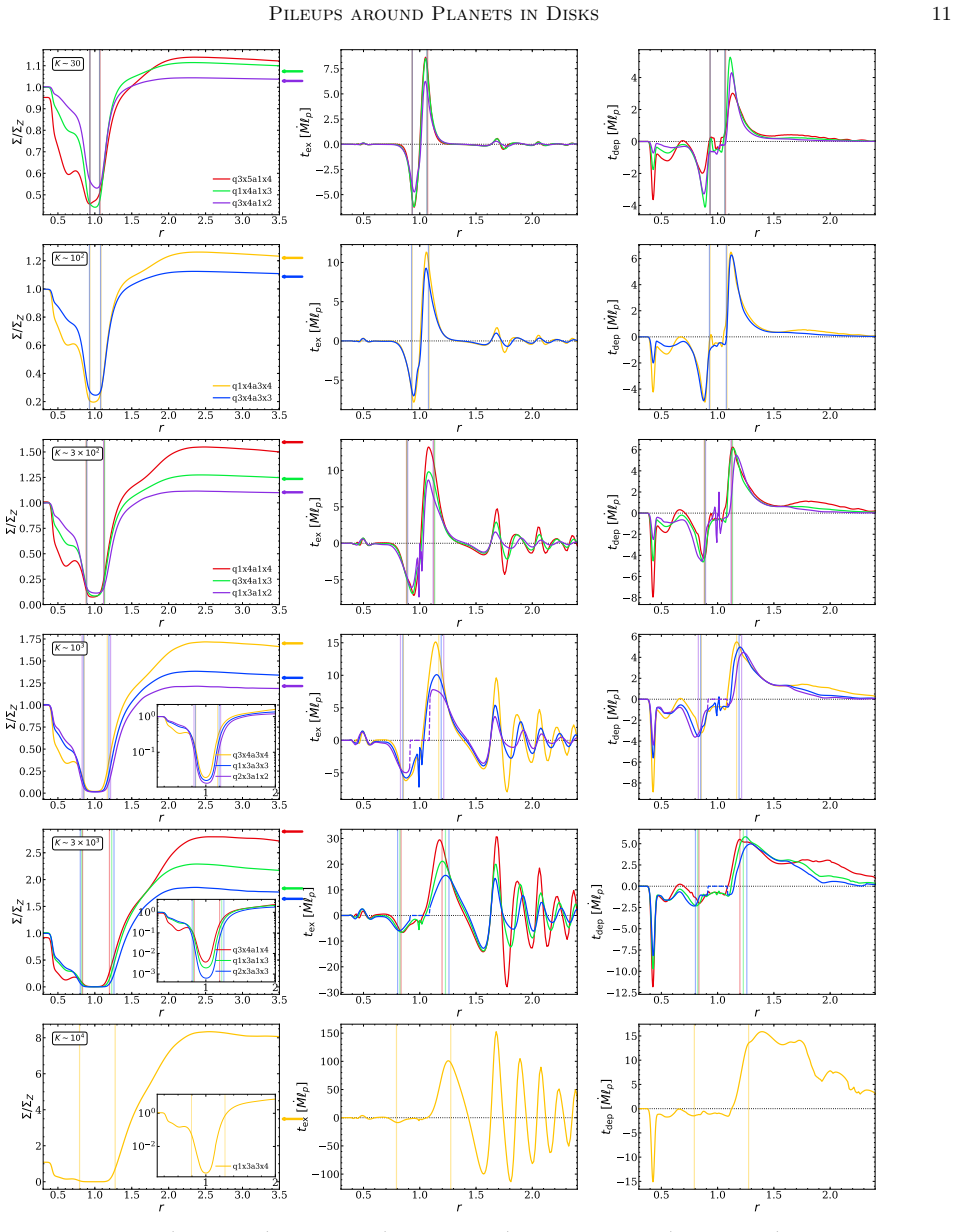
The load-bearing object is $\Delta T$, the total two-sided torque the planet applies to the disk, defined as the integral of the excited torque density over all radii. The argument separates angular-momentum transport into wave excitation, wave propagation, and deposition: waves carry angular momentum from Lindblad resonances near the planet to where they damp, and the deposited torque density $t_{\rm dep}$ shapes the surface-density profile through the viscous-steady-state equation $F_\nu = \dot M\ell + \int^r t_{\rm dep}\,dr'$. Far from the planet this yields $\Sigma = \Sigma_Z$ inside and $\Sigma = \Sigma_Z(1+\Delta T/(\dot M\ell))$ outside, so $\Delta T$ sets the pileup height, and the same $\Delta T$ enters the migration formula. The numerical boundary conditions are chosen to match these steady-state solutions so the pileup can survive.
What would settle it
Run a viscous-steady-state simulation with the inner boundary moved to a much smaller radius, or with the inner wave-killing zone removed, and check whether $\Delta T/(\dot M\ell_p)$ and the exterior pileup level stay within the paper's quoted accuracy; if they shift significantly, the empirical fit and the derived migration rate are biased by the boundary treatment.
Extended reading notes
Core claim
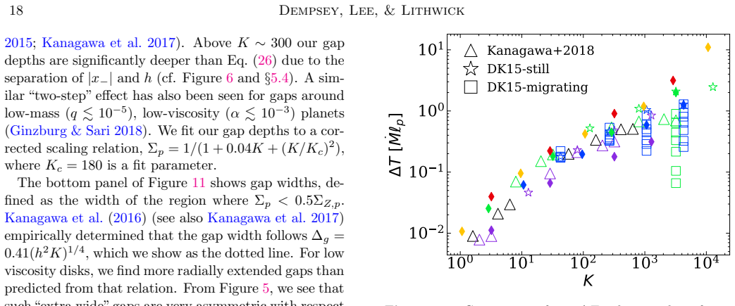
In a low-mass disk, a gap-opening planet acts as a leaky dam: gas keeps accreting inward across the planet's orbit, but the angular momentum the planet deposits makes the exterior disk denser than a planet-free disk by the factor $1+\Delta T/(\dot M\ell_p)$. The paper shows that the same two-sided torque $\Delta T$ fixes the migration rate through $\dot r_p/r_p = -2\Delta T/(M_p\ell_p)$, so in viscous steady state the planet is not locked to the disk's viscous accretion but migrates at a rate set by the torque balance. For moderately deep gaps the paper derives $\Delta T$ from a gap-depth argument based on the torque cutoff, matching simulations; for deep gaps the simulations give an empirical scaling, roughly $\Delta T/(\dot M\ell_p)\sim 4(q/\alpha)$, so the deep-gap migration rate becomes nearly independent of planet mass and viscosity. These results explain why earlier 2D simulations missed the pileup (incorrect boundary conditions) and why 1D local-deposition models overpredicted it dramatically.
Load-bearing premise
The load-bearing premise is that the measured two-sided torque $\Delta T$ is set by wave excitation close to the planet, so the artificial inner boundary and angular-momentum-conserving wave-killing zone that distort the inner disk profile do not change the pileup or migration rate.
Editorial extensions
If this is right
- Gas exterior to a gap-opening planet in a low-mass disk should sit above the planet-free profile by $1+\Delta T/(\dot M\ell)$, giving a directly observable pileup that traces the planet-disk torque.
- The deep-gap migration rate is nearly independent of planet mass and disk viscosity, scaling mainly with the disk-to-star mass ratio, in contrast to classical Type-II 'locked to the disk' migration.
- The Type-I and Type-II migration rates join smoothly near $K\sim100$, so one torque formula covers the transition from low-mass to massive planets in low-mass disks.
- Published 2D simulations that held all fluid quantities at their initial values at the boundaries would not produce the pileup, while 1D local-deposition models overpredict it by factors like $e^{200}$ at $K\sim10^4$.
Reading between the lines
- Going beyond the paper: if an observed ring or cavity in a directly imaged disk is a pileup, comparing the brightness contrast at large radius with independent estimates of $\dot M$ and $\alpha$ could break the degeneracy between planet mass and viscosity that a single gap-depth measurement carries.
- Going beyond the paper: the empirical deep-gap scaling $\Delta T/(\dot M\ell)\propto q/\alpha$ suggests the pileup may grow only sub-linearly as $K$ increases, so the leaky-dam picture implies an upper bound on pileup that could be tested by pushing simulations beyond $K\sim10^4$.
- Going beyond the paper: a migration rate that is nearly independent of disk viscosity would mean giant-planet migration timescales in low-mass disks are no longer tied to the disk's viscous time, a shift that would change interpretations of observed exoplanet orbits.
Signed reviews
Editorial analysis
A structured set of objections, weighed in public.
Referee Report
Summary. The paper studies planet-disk interaction in the low-disk-mass limit, where the planet's migration is slower than the disk's viscous evolution and the disk can be treated as passing through a sequence of viscous steady states (VSS). The authors introduce boundary conditions that allow 2D hydrodynamical simulations to reach VSS, and they show that the two-sided planet torque ΔT controls both the exterior pileup and the planet's migration rate. For moderately deep gaps they derive a first-principles prediction for ΔT (Eqs. 21-29) that agrees with their simulations at K ≲ 100. For deeper gaps they present an empirical power-law fit (Eq. 32) and use it to obtain a new Type-II migration rate (Eq. 38) that is nearly independent of planet mass and viscosity. They also show that previous 1D local-deposition models greatly overpredict the pileup, and they identify the difficulty of constructing a complete theory of very deep gaps.
Significance. If the central claims hold, the paper provides a clean organizing framework for planet-disk interaction in low-mass disks: a single quantity, ΔT, links the observable pileup, the gap profile, and the migration rate. The torque bookkeeping is carefully checked (Fig. 4), the moderate-gap prediction matches the simulations without fitted coefficients, and the resolution study gives 10% average (30% worst) agreement in ΔT. The paper also gives a clear explanation of why previous 1D local-deposition models fail and why earlier 2D simulations missed the pileup. These are substantial contributions. However, the headline deep-gap result, the new Type-II migration rate, rests on an empirical fit whose selection and regime boundaries are not robustly justified, so the quantitative deep-gap conclusions are not yet established at the same level as the moderate-gap results.
major comments (3)
- [Section 4.5 and Eq. (32); used in Section 5.1, Eq. (38)] The empirical fit underlying the deep-gap migration rate is not restricted to the deep-gap regime. Eq. (32) is fitted to all runs with q > 10^-4, which includes many K < 100 points where the moderate-gap scaling ΔT ∝ q^2/α (Eq. 29) is known to hold and has a different dependence. The deepest-gap point q1x3a3x4 (K = 1.07e4, ΔT/(Ṁ l_p) = 11.0) is excluded as 'unusually large,' yet this is the most extreme and most observationally relevant point. At the quoted fit this point lies a factor of roughly 2 above the prediction, so its exclusion is consequential. Since Eq. (38) and the claim of near-independence from q and α follow directly from the fitted exponents q^1.05 and α^-0.91, the authors should refit using only K ≳ 100 points, report the fit with and without q1x3a3x4, and show how Eq. (38) changes. As written, the central deep-gap result is not robust to reasonable changes in the fitting procedure.
- [Section 4.1, Section 5.4, and Table 1] The assertion that the artificial inner wave-killing zone has 'negligible effect on the value of ΔT' is load-bearing for the deep-gap results, but it is not demonstrated by a domain-size or wave-killing-zone test. For the highest-K runs the gap extends past the inner boundary (Section 5.2 and Fig. 11), and the deepest-gap point q1x3a3x4 is also the point with the largest low-resolution deviation in ΔT (14.2 vs. 11.0 in Table 1). Because ΔT at high K is the small difference of larger one-sided torques, a test that moves ri,wkz inward (or enlarges the domain) is needed to show that the deepest-gap pileup and the fitted Eq. (32) are not biased by the inner boundary treatment.
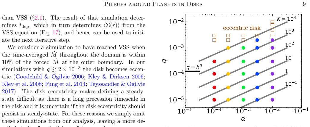
- [Section 3.2 and Section 5.1] The VSS convergence criterion is a 10% global consistency of Ṁ, and runs that become eccentric or fail to converge are omitted from the analysis. This selection could bias the fitted q-α scaling if convergence correlates with q or α, which is plausible given that the deepest-gap and lowest-α runs are the most expensive and the least converged. The authors should show that the excluded or longer-time runs do not change the fitted exponents in Eq. (32), or at least quantify how the fit depends on the adopted convergence threshold.
minor comments (4)
- [Section 4.5, Eq. (32)] The displayed uncertainty on the coefficient in Eq. (32) is garbled ('4.36.6 2.8'); the statistical errors on the exponents are quoted, but the notation should be cleaned up and the covariance of the fitted parameters should be reported.
- [Section 3.1 and Fig. 4] The description of the inner and outer wave-killing zones would be clearer if the radii ri,wkz and ro,wkz were marked consistently on all panels of Figure 4; currently the reader must look back and forth between the text and the figure.
- [Section 5.1, Eq. (38)] The statement that the deep-gap migration rate is 'roughly independent of their mass and the disk's viscosity' is only as good as the fitted exponents in Eq. (32). A short sensitivity statement around Eq. (38), showing how the q^0.05 α^0.09 factors change under the alternative fits suggested above, would help the reader assess the strength of this claim.
- [Section 7, Open Questions] The paper is commendably explicit about the limitations of the deep-gap theory and about the inner-boundary issue. These statements should be retained in the final version; they correctly frame the empirical fit as a starting point rather than a complete theory.
Circularity Check
Minor non-independent consistency check in the deep-gap one-sided torque comparison, but the central VSS derivation and moderate-gap theory are not circular.
-
fitted input called prediction
[Section 5.4, Eq. (31) and Figure 14]
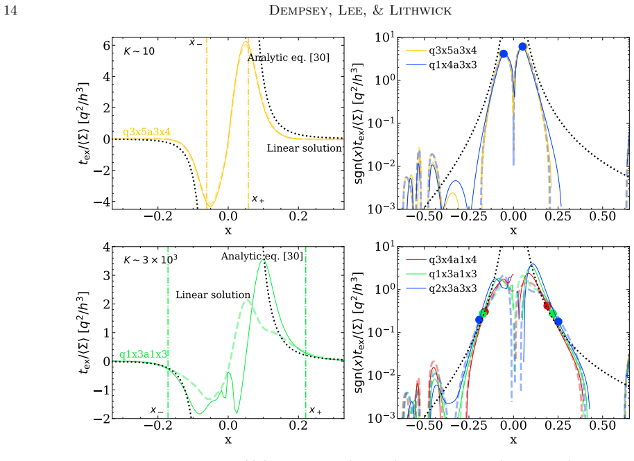
"Figure 14 compares this prediction for T± with what is found in the simulations, where the “prediction” makes use of the values of x± and Σ± extracted from the simulations."
The one-sided torques T± are measured from the same hydrodynamical simulations that supply the inputs x± and Σ±. Equation (31) evaluates the analytic torque formula at those measured peak locations and peak surface densities, and Figure 14 then compares the result with the measured T±. The agreement is therefore a consistency check of the approximate torque formula, not an independent, out-of-sample prediction of the deep-gap torques. The paper itself marks the word “prediction” with scare quotes, and this step is not used to determine the deep-gap ΔT or the migration rate; those come directly from the simulation measurements and the empirical fit in Eq. (32). Hence the circularity is real but minor and non-load-bearing.
full rationale
The main derivation chain is not circular. The VSS relations, Eqs. (17)–(19), follow from angular-momentum conservation, and the moderate-gap torque prediction, Eqs. (21)–(29), is obtained from linear theory with the coefficients C± computed in Appendix B rather than fitted to the simulations; it is then checked against the simulations and agrees at K ≲ 100. The deep-gap migration rate, Eq. (38), is not presented as a first-principles prediction: the paper states “Using that fit to ΔT, the migration rate is,” and Eq. (38) is the algebraic consequence of the empirical power-law fit Eq. (32). That is an honest simulation-based result, not a fitted parameter renamed as a prediction. The only place where a “prediction” is built from the same simulation’s own outputs is the Eq. (31)/Figure 14 comparison of one-sided torques, which is non-independent but does not support the central pileup or migration claims. The self-citations (Lee 2016; Lee et al. 2019) are used for technical sub-points, not as load-bearing justification, and no uniqueness theorem is imported from the authors’ prior work. Concerns about excluding the K ∼ 10^4 point or omitting eccentric/non-converged runs are statistical robustness issues, not circularity. Overall, the central moderate-gap theory is self-contained, and the deep-gap results are transparently empirical.
Assumptions & free parameters
free parameters (2)
- Deep-gap ΔT fit: normalization and exponents (Eq. 32) =
A = 4.36 (range 2.8 to 6.6), exponent on q = 1.05 ± 0.06, exponent on α = -0.91 ± 0.04
- Gap depth fit parameter K_c =
K_c = 180
assumptions (5)
- domain assumption The disk is locally isothermal, P = c_s^2 Σ with c_s = h r Ω_K, with h = 0.05 fixed.
- domain assumption The planet is on a fixed circular orbit and does not accrete material; migration is inferred from the torque on a stationary planet.
- domain assumption The waves' angular momentum deposition (t_dep) controls the surface density profile, and the standard Lindblad torque formula with the leading asymmetry (Eq. 30) is applicable at the excitation sites x±.
- domain assumption The 2D hydrodynamical treatment with a softened planet potential (softening 0.6h) captures the relevant physics; 3D effects are neglected.
- ad hoc to paper The imposed boundary conditions with wave-killing zones that damp only v_r (conserving angular momentum) drive the disk to the true VSS, and the artificial inner wave-killing zone does not affect ΔT.
Cite this review
Pith. "Pith review of Pileups and Migration Rates for Planets in Low Mass Disks." pith.science (2026). https://pith.science/paper/UBE5W4CG
@misc{pith2026190802326,
  author       = {Pith},
  title        = {Pith review of: Pileups and Migration Rates for Planets in Low Mass Disks},
  year         = {2026},
  howpublished = {\url{https://pith.science/paper/UBE5W4CG}},
  note         = {Machine review of arXiv:1908.02326}
}
read the original abstract
We investigate how planets interact with viscous accretion disks, in the limit that the disk is sufficiently low mass that the planet migrates more slowly than the disk material. In that case, the disk's surface density profile is determined by the disk being in viscous steady state (VSS), while overflowing the planet's orbit. We compute the VSS profiles with 2D hydrodynamical simulations, and show that disk material piles up behind the planet, with the planet effectively acting as a leaky dam. Previous 2D hydrodynamical simulations missed the pileup effect because of incorrect boundary conditions, while previous 1D models greatly overpredicted the pileup due to the neglect of non-local deposition. Our simulations quantify the magnitude of the pileup for a variety of planet masses and disk viscosities. We also calculate theoretically the magnitude of the pileup for moderately deep gaps, showing good agreement with simulations. For very deep gaps, current theory is inadequate, and we show why and what must be understood better. The pileup is important for two reasons. First, it is observable in directly imaged protoplanetary disks, and hence can be used to diagnose the mass of a planet that causes it or the viscosity within the disk. And second, it determines the planet's migration rate. Our simulations determine a new Type-II migration rate (valid for low mass disks), and show how it connects continuously with the well-verified Type-I rate.
Figures


Figures from the paper (13 more)






Reference graph
Works this paper leans on
-
[1]
, " * write output.state after.block = add.period write newline
ENTRY address archivePrefix author booktitle chapter doi edition editor eprint howpublished institution journal key month number organization pages publisher school series title misctitle type volume year version url label extra.label sort.label short.list INTEGERS output.state before.all mid.sentence after.sentence after.block FUNCTION init.state.consts ...
-
[2]
write newline
" write newline "" before.all 'output.state := FUNCTION format.url url empty "" new.block "" url * "" * if FUNCTION format.eprint eprint empty "" archivePrefix empty "" archivePrefix "arXiv" = new.block " " eprint * " " * new.block " " eprint * " " * if if if FUNCTION format.doi doi empty "" " " doi * " " * if FUNCTION format.pid doi empty eprint empty ""...
-
[3]
thebibliography [1] 20pt to REFERENCES 6pt =0pt 10pt plus 3pt =0pt =0pt =1pt plus 1pt =0pt =0pt -12pt =13pt plus 1pt =20pt =13pt plus 1pt \@M =10000 =-1.0em =0pt =0pt 0pt =0pt =1.0em @enumiv\@empty 10000 10000 `\.\@m \@noitemerr \@latex@warning Empty `thebibliography' environment \@ifnextchar \@reference \@latexerr Missing key on reference command Each re...
-
[4]
L., Perez, L
ALMA Partnership , Brogan, C. L., Perez, L. M., et al. 2015, , 808, L3
2015
-
[5]
M., Wilner, D
Andrews, S. M., Wilner, D. J., Espaillat, C., et al. 2011, , 732, 42
2011
-
[6]
M., Wilner, D
Andrews, S. M., Wilner, D. J., Zhu, Z., et al. 2016, , 820, L40
2016
-
[7]
Andrews, S. M., Huang, J., P \'e rez, L. M., et al. 2018, , 869, L41
work page 2018
-
[8]
J.\ 2010, Astrophysics of Planet Formation (Cambridge: Cambridge University Press)
Armitage, P. J.\ 2010, Astrophysics of Planet Formation (Cambridge: Cambridge University Press)
work page 2010
Show all 84 references
-
[9]
1993, , 419, 155
Artymowicz, P. 1993, , 419, 155
1993
-
[10]
J., et al
Baruteau, C., Crida, A., Paardekooper, S. J., et al. 2014, in Protostars and Planets VI, ed. H. Beuther et al. (Tucson, AZ: Univ. Arizona Press), 667
2014
-
[11]
Ben \' tez-Llambay, P., & Masset, F. S. 2016, , 223, 11
2016
-
[12]
2006, , 181, 587
Crida, A., Morbidelli, A., & Masset, F. 2006, , 181, 587
2006
-
[13]
2016, , 595, A114
de Boer, J., Salter, G., Benisty, M., et al. 2016, , 595, A114
2016
-
[14]
G., Artymowicz, P., et al
de Val-Borro, M., Edgar, R. G., Artymowicz, P., et al. 2006, , 370, 529
2006
-
[15]
E., & Salyk, C
Dodson-Robinson, S. E., & Salyk, C. 2011, , 738, 131
2011
-
[16]
2017, , 835, 146
Dong, R., & Fung, J. 2017, , 835, 146
2017
-
[17]
2018, , 866, 110
Dong, R., Li, S., Chiang, E., & Li, H. 2018, , 866, 110
2018
-
[18]
R., Stone, J
Dong, R., Rafikov, R. R., Stone, J. M., et al.\ 2011, , 741, 56
2011
-
[19]
Duffell, P. C. 2015, , 807, L11
2015
- [20]
-
[21]
C., Haiman, Z., MacFadyen, A
Duffell, P. C., Haiman, Z., MacFadyen, A. I., D'Orazio, D. J., & Farris, B. D. 2014, , 792, L10
2014
-
[22]
C., & MacFadyen, A
Duffell, P. C., & MacFadyen, A. I. 2013, , 769, 41
2013
-
[23]
2015, , 574, A52
D \"u rmann, C., & Kley, W. 2015, , 574, A52
2015
-
[24]
Edgar, R. G. 2007, , 663, 1325
2007
-
[25]
2014, in Protostars and Planets VI, ed
Espaillat, C., Muzerolle, J., Najita, J., et al. 2014, in Protostars and Planets VI, ed. H. Beuther et al. (Tucson, AZ: Univ. Arizona Press), 497
2014
-
[26]
R., et al
Fedele, D., Carney, M., Hogerheijde, M. R., et al. 2017, , 600, A72
2017
-
[27]
2016, , 832, 105
Fung, J., & Chiang, E. 2016, , 832, 105
2016
-
[28]
2014, , 782, 88
Fung, J., Shi, J.-M., & Chiang, E. 2014, , 782, 88
2014
-
[29]
2018, , 479, 1986
Ginzburg, S., & Sari, R. 2018, , 479, 1986
2018
-
[30]
1979, , 233, 857
Goldreich, P., & Tremaine, S. 1979, , 233, 857
1979
-
[31]
1980, , 241, 425
---. 1980, , 241, 425
1980
-
[32]
2006, , 368, 1123
Goodchild, S., & Ogilvie, G. 2006, , 368, 1123
2006
-
[33]
Goodman, J., & Rafikov, R. R. 2001, , 552, 793
2001
-
[34]
Greenberg, R.\ 1983, , 53, 207
1983
-
[35]
Y., Bohn, A
Haffert, S. Y., Bohn, A. J., de Boer, J., et al. 2019, Nature Astronomy, 50, 211
2019
-
[36]
2016, , 117, 251101
Isella, A., Guidi, G., Testi, L., et al. 2016, , 117, 251101
2016
-
[37]
B., Papaloizou, J
Ivanov, P. B., Papaloizou, J. C. B., & Polnarev, A. G. 1999, , 307, 79
1999
-
[38]
D., Muto, T., Tanaka, H., et al
Kanagawa, K. D., Muto, T., Tanaka, H., et al. 2015 a , , 806, L15
2015
-
[39]
D., Tanaka, H., Muto, T., & Tanigawa, T
Kanagawa, K. D., Tanaka, H., Muto, T., & Tanigawa, T. 2017, , 69, 97
2017
-
[40]
D., Tanaka, H., Muto, T., Tanigawa, T., & Takeuchi, T
Kanagawa, K. D., Tanaka, H., Muto, T., Tanigawa, T., & Takeuchi, T. 2015 b , , 448, 994
2015
-
[41]
D., Tanaka, H., & Szuszkiewicz, E
Kanagawa, K. D., Tanaka, H., & Szuszkiewicz, E. 2018, , 861, 140
2018
-
[42]
2006, , 447, 369
Kley, W., & Dirksen, G. 2006, , 447, 369
2006
-
[43]
Kley, W., & Nelson, R. P. 2012, , 50, 211
2012
-
[44]
Kley, W., Papaloizou, J. C. B., & Ogilvie, G. I. 2008, , 487, 671
2008
-
[45]
2012 a , , 427, 2660
Kocsis, B., Haiman, Z., & Loeb, A. 2012 a , , 427, 2660
2012
-
[46]
2012 b , , 427, 2680
---. 2012 b , , 427, 2680
2012
-
[47]
G., & Pollack, J
Korycansky, D. G., & Pollack, J. B. 1993, , 102, 150
1993
-
[48]
2016, , 832, 166
Lee, W.-K. 2016, , 832, 166
2016
-
[49]
M., & Lithwick, Y.\ 2019, , 882, L11
Lee, W.-K., Dempsey, A. M., & Lithwick, Y.\ 2019, , 882, L11
2019
-
[50]
Lin, D. N. C., & Papaloizou, J. 1986 a , , 307, 395
1986
-
[51]
1986 b , , 309, 846
---. 1986 b , , 309, 846
1986
-
[52]
Lin, D. N. C., & Papaloizou, J. C. B. 1993, in Protostars and Planets III, ed. E. H. Levy & J. I. Lunine (Tucson, AZ: Univ. Arizona Press), 749
1993
-
[53]
T., & Shapiro, S
Liu, Y. T., & Shapiro, S. L. 2010, , 82, 123011
2010
-
[54]
Lynden-Bell, D., & Pringle, J. E. 1974, , 168, 603
1974
-
[55]
I., & Stevenson, D
Lunine, J. I., & Stevenson, D. J.\ 1982, , 52, 14
1982
-
[56]
2000, , 141, 165
Masset, F. 2000, , 141, 165
2000
-
[57]
2004, , 606, 520
Menou, K., & Goodman, J. 2004, , 606, 520
2004
-
[58]
J., & Lai, D
Miranda, R., Mu \ n oz, D. J., & Lai, D. 2017, , 466, 1170
2017
-
[59]
Miranda, R., & Rafikov, R. R. 2019, , 878, L9
2019
-
[60]
M \"u ller, T. W. A., Kley, W., & Meru, F. 2012, , 541, A123
2012
-
[61]
J., Miranda, R., & Lai, D.\ 2019, , 871, 84
Mu \ n oz, D. J., Miranda, R., & Lai, D.\ 2019, , 871, 84
2019
-
[62]
K., & Inutsuka, S.-i
Muto, T., Suzuki, T. K., & Inutsuka, S.-i. 2010, , 724, 448
2010
-
[63]
Ogilvie, G. I. 2008, , 388, 1372
2008
-
[64]
I., & Lubow, S
Ogilvie, G. I., & Lubow, S. H. 2002, , 330, 950
2002
-
[65]
J., & Papaloizou, J
Paardekooper, S. J., & Papaloizou, J. C. B. 2009, , 394, 2283
2009
-
[66]
R.\ 2012, , 758, 33
Petrovich, C., & Rafikov, R. R.\ 2012, , 758, 33
2012
-
[67]
Rafikov, R. R. 2002 a , , 569, 997
2002
-
[68]
R.\ 2002 b , , 572, 566
Rafikov, R. R.\ 2002 b , , 572, 566
2002
-
[69]
R.\ 2013, , 774, 144
Rafikov, R. R.\ 2013, , 774, 144
2013
-
[70]
R.\ 2016, , 827, 111
Rafikov, R. R.\ 2016, , 827, 111
2016
-
[71]
R., & Petrovich, C.\ 2012, , 747, 24
Rafikov, R. R., & Petrovich, C.\ 2012, , 747, 24
2012
-
[72]
Robert, C. M. T., Crida, A., Lega, E., M \'e heut, H., & Morbidelli, A. 2018, , 617, A98
2018
-
[73]
I., & Sunyaev, R
Shakura, N. I., & Sunyaev, R. A. 1973, , 24, 337
1973
-
[74]
Syer, D., & Clarke, C. J. 1995, , 277, 758
1995
-
[75]
Tanaka, H., Takeuchi, T., & Ward, W. R. 2002, , 565, 1257
2002
-
[76]
Tang, Y., MacFadyen, A., & Haiman, Z.\ 2017, , 469, 4258
2017
-
[77]
2007, , 667, 557
Tanigawa, T., & Ikoma, M. 2007, , 667, 557
2007
-
[78]
Teyssandier, J., & Ogilvie, G. I. 2017, , 467, 4577
2017
-
[79]
F., Bruderer, S., et al
van der Marel, N., van Dishoeck, E. F., Bruderer, S., et al. 2016, , 585, A58
2016
-
[80]
Ward, W. R. 1997, , 126, 261
1997
-
[81]
P., & Cieza, L
Williams, J. P., & Cieza, L. A. 2011, , 49, 67
2011
-
[82]
2018, , 869, L47
Zhang, S., Zhu, Z., Huang, J., et al. 2018, , 869, L47
2018
-
[83]
P., Dong, R., Espaillat, C., & Hartmann, L
Zhu, Z., Nelson, R. P., Dong, R., Espaillat, C., & Hartmann, L. 2012, , 755, 6
2012
-
[84]
P., Hartmann, L., Espaillat, C., & Calvet, N
Zhu, Z., Nelson, R. P., Hartmann, L., Espaillat, C., & Calvet, N. 2011, , 729, 47
2011
Reviewed August 14, 2026 · model on record in the stance chip above.
Discussion (0). Continue with ORCID to comment.