REVIEW 3 major objections 4 minor 74 references
Interpreting learning dynamics of autoencoders: Transient scaling and emerging concepts of the Ising model
T0 review · 3 major / 4 minor · reviewed 2026-08-02 · deepseek-v4-flash
Pith's one-line read This paper claims that autoencoders trained on Ising-model spin configurations learn macroscopic concepts in a fixed order — first magnetization, then energy — and that this order can be read off from reconstruction losses decomposed across
desk verdict A substantial empirical study of scale-resolved autoencoder dynamics whose headline 'energy regime' is contradicted by its own Fig. 23; the magnetization result is solid, but the central claim needs rework. read the letter →
The pith
A machine-rendered reading of the paper's core claim, the machinery that carries it, and where it could break.
The reading
What carries the argument
The load-bearing tool is a scale-resolved loss: reconstruction error is computed not just on raw pixels but on averages over square neighborhoods (kernels) of growing size, turning the loss into a function of the coarse-graining scale. A second probe is self-recursion: the trained network is applied to its own output to generate latent-space trajectories; a rank correlation between latent distances and an observable's difference measures whether the latent space is topologically ordered by that concept. Together these let the authors watch the order in which macroscopic concepts form.
What would settle it
Evaluate the coarse-grained validation losses separately for each of the fifteen temperatures. If the global minimum in the largest-scale loss, and the subsequent rise, appears only at temperatures far from the training set (T ≥ 2.5) and not at the five training temperatures, the claimed magnetization-then-energy sequence and bottleneck-induced trade-off would not hold; equivalently, train and validate on the same critical temperatures and check whether the trade-off persists.
Extended reading notes
Core claim
The central claim is that, when the mean-squared reconstruction error is averaged over square patches of growing size on the 16x16 lattice, successful training shows two distinct phases: a magnetization phase in which losses at all scales decrease monotonically and the output is a spatially uniform version of the input, followed by an energy phase in which small-scale structure is resolved and losses become scale-dependent. The transition is marked by a minimum in large-scale losses, which then rise as small-scale features improve — a representational trade-off that the authors attribute to the information bottleneck. Deep autoencoders (depth 16) trained at learning rates of 1e-4 or 1e-3 nev
Load-bearing premise
The magnetization-to-energy sequence is read off from validation losses averaged over all fifteen temperatures, even though training used only the five critical-adjacent temperatures, so the apparent trade-off could be an artifact of distribution shift rather than an intrinsic bottleneck effect.
Editorial extensions
If this is right
- For shallow models (depths 1 and 4), learning global spin averages before local fluctuations appears to be a robust ordering, so simpler statistics of the data are mastered before finer correlations.
- The large-scale loss minimum and subsequent rise constitutes a scale-resolved signature of a representational trade-off, and its strength decreases as the bottleneck grows.
- Deep models at intermediate and fast learning rates exhibit an arrested regime in which they output only the dataset average; this regime is identifiable from flat, scale-invariant run variance.
- The robustness of the latent-space topological ordering under recursion can serve as an indicator that a concept has actually been learned, not merely that the reconstruction loss dropped.
- The joint output distribution of magnetization and energy shows that high-energy validation configurations are systematically underestimated, indicating that the bottleneck limits resolution of small-scale features even in successful models.
Reading between the lines
- If the magnetization-then-energy order reflects the data's correlation structure rather than anything specific to Ising systems, the same scale-resolved loss probe could be used on images, turbulence data, or other multiscale datasets to detect when a model is about to resolve finer scales.
- The recursion-dynamics measurement could double as a practical monitoring heuristic: a latent space whose topology for a target concept is stable under recursion may be a better early-stopping signal than the raw validation loss.
- The per-temperature validation analysis lives only in the supplementary material; using it in the main narrative would clarify whether the trade-off is intrinsic or a distribution-shift artifact. This is my inference, not the paper's claim.
- One could test whether an explicitly curriculum-driven training schedule — feeding low-temperature samples first, then progressively warmer ones — reproduces or accelerates the magnetization-to-energy sequence, which would suggest the emergent order is an implicit curriculum.
Editorial analysis
A structured set of objections, weighed in public.
Referee Report
Summary. The paper studies how deterministic ReLU autoencoders trained on 2D Ising spin configurations learn macroscopic concepts, using spatially coarse-grained validation losses for magnetization and energy. Based on 972 training runs, it claims that learning proceeds through two sequential dynamical regimes — first magnetization, then energy — and that depth, width, and learning rate control the transition, with deep models trained at moderate/fast rates becoming arrested before the energy regime. The paper also introduces an analysis of self-recursive latent dynamics and Spearman-rank 'topological ordering' to connect reconstruction errors to internal concept formation.
Significance. If the central claim were established, the paper would provide a substantial empirical contribution: a hyperparameter-controlled, scale-resolved picture of concept formation in autoencoders on a physically grounded dataset. Strengths include the large ablation study, publicly available code/checkpoints, comparisons to trivial baselines (dataset mean and sample mean), and the fact that the two regimes are measured rather than fitted. However, the central energy-regime claim is directly contradicted by the paper's own Fig. 23 and Appendix §VI E 3, which state that no energy loss at any scale consistently decreases over training. This internal inconsistency prevents acceptance of the paper in its current form; the remaining distribution-shift confound also weakens the causal interpretation of the magnetization-to-energy trade-off.
major comments (3)
- [Abstract; §V; §VI E 3 and Fig. 23] The central claim is internally inconsistent. The Abstract states that there is a regime 'in which energy is learned across scales,' and §V asserts that 'the magnetization or the energy losses decrease monotonically across all scales.' But §VI E 3 says, describing Fig. 23 for the same MB8DXWX ensemble used in the main narrative, 'not a single loss on any of the scales in Fig. 23 consistently decreases over training. Notably, the losses even increase compared to the randomly initialized model in most cases.' The caption adds that final average energy loss is larger than initial for most models, except at d=4. If 'decrease across all scales' means temporal decrease at each kernel size, Fig. 23 falsifies the energy regime as stated; if it means the static ordering of loss versus kernel size, that is not a sequential dynamical regime. Either way, the strongest concrete assertion in §V is uns
- [§III A 2; §IV B 2; §IV B 3; §V] The magnetization-to-energy sequence and the bottleneck-causes-trade-off interpretation are confounded by a validation distribution shift. Training uses only the five temperatures near T_c, while validation losses are averaged over all 15 temperatures. The paper itself notes in §IV B 3 that the highest-energy samples 'are only present in the validation data.' The rise of the large-scale loss after its minimum in Fig. 6 could therefore be an artifact of the model degrading on far-from-training temperatures, rather than a bottleneck-induced representational trade-off. Per-temperature validation curves are not used in the main narrative. Without ruling out distribution shift, the claim in §V that 'the bottleneck constraint is the cause of the trade-off' is not established. The authors should either show per-temperature versions of the key scale-resolved curves or explicitly qualify the trad
- [§IV C 2 and Fig. 10] The concluding sentence of §IV C 2 states that stability under recursion 'is a prerequisite for consistently improving their reconstruction.' This causal claim is stronger than what the Spearman-rank analysis supports: the analysis shows a temporal concurrence between high stable rank correlation and decreasing magnetization loss, but correlation at the same training checkpoints does not establish precedence or causation. This is not the primary claim of the paper, but the wording should be softened to 'associated with' or 'precedes in the observed runs' unless a temporal ordering is demonstrated.
minor comments (4)
- [Abstract] Grammar/punctuation issues: 'The first exhibits error fluctuations ordered to scale and learns global averages only; The second' uses a semicolon followed by a capital 'The,' and the sentence is run-on. Recommend copyediting.
- [§IV B 2] The notation for coarse-grained magnetization is used as M(k) but the definition of the kernel set K_k^i is not fully specified in the main text; please clarify the relation between kernel size k and the 'a×a' notation in L_{M(k)} = L_{k=a×a}(...).
- [Fig. 20 caption] The caption refers to 'w=1025 models'; the main text and Table I only define widths 256, 512, and 1024. This is likely a typo and should be corrected.
- [§VI E 3 / Fig. 23] The appendix's observation that only d=4 models show a final average energy loss lower than the initial loss is important; it should be discussed in the main text, not buried in a caption, because it bears directly on the energy-regime claim.
Circularity Check
No circularity found: the regime claims are empirical measurements from an external physical ground truth, not fitted parameters; the internal Fig. 23 inconsistency is a correctness issue, not circularity.
full rationale
Walked the derivation chain. The core result is an empirical decomposition of validation reconstruction losses by coarse-graining scale (Fig. 6, Fig. 23) and an ablation over depth/width/learning rate. The magnetization and energy observables are taken from the Ising Hamiltonian (Sec. II B) and the local-gradient definition (Sec. VI E 3), which are external ground truths, not fitted parameters. No parameter is fitted to the data and then renamed as a prediction; the 'regimes' are read off the measured loss curves, and the hyperparameter dependence is established by direct comparison across the 972-run grid. The self-citations ([14,23,26,48]) are contextual or data-repository references and are not load-bearing for the regime claim. I specifically checked the claim in Sec. V that 'the magnetization or the energy losses decrease monotonically across all scales' against Sec. VI E 3 / Fig. 23, where the paper states "not a single loss on any of the scales in Fig. 23 consistently decreases over training. Notably, the losses even increase compared to the randomly initialized model in most cases." That is an internal inconsistency in the empirical support for the energy-regime claim and should be resolved (e.g., by distinguishing 'decrease over training time' from 'decrease with kernel size' or by restricting the claim to d=4), but it is a correctness/data-interpretation issue, not circularity: the claim is not equivalent to its inputs by construction. No step in the paper reduces a predicted quantity to a fitted quantity or to an unverified self-citation. Therefore no significant circularity; score 0.
Assumptions & free parameters
free parameters (4)
- Training temperature set =
{2.1, 2.2, 2.27, 2.3, 2.4}
- Base learning rates =
{1e-5, 1e-4, 1e-3}
- Learning-rate schedule =
linear warmup to step 100, cosine decay to 0 at step 100,000
- Coarse-graining kernel sizes =
3x3 to 13x13 (approximate; exact set not enumerated)
assumptions (6)
- domain assumption MCMC (Glauber) sampling with 1e6-step thinning and multiple seeds yields independent Boltzmann-distributed Ising configurations
- domain assumption Validation loss averaged over all 15 temperatures measures whether observables are 'learned'
- domain assumption 'Regimes' and 'arrest' are identified by visual inspection of loss curves without quantitative thresholds or statistical tests
- ad hoc to paper Self-recursive application of the trained autoencoder defines an 'intrinsic dynamic' whose fixed points/cycles reflect internal concept formation
- ad hoc to paper Spearman correlation between latent distance and observable difference measures 'topological ordering' of a concept
- domain assumption Learning dynamics can be described by a small set of macroscopic observables (magnetization, energy) of the data-generating process
Cite this review
Pith. "Pith review of Interpreting learning dynamics of autoencoders: Transient scaling and emerging concepts of the Ising model." pith.science (2026). https://pith.science/paper/UG6IQGW6
@misc{pith2026260710285,
  author       = {Pith},
  title        = {Pith review of: Interpreting learning dynamics of autoencoders: Transient scaling and emerging concepts of the Ising model},
  year         = {2026},
  howpublished = {\url{https://pith.science/paper/UG6IQGW6}},
  note         = {Machine review of arXiv:2607.10285}
}
read the original abstract
We study how unsupervised autoencoders trained on microscopic spin configurations from the Ising model learn macroscopic, theory-relevant variables underlying the data-generating process. We quantify learning across multiple spatial (coarse-graining) scales and reveal two distinct dynamical regimes that appear sequentially, controlled by the main hyperparameters (model depth, width, and learning rate): one in which magnetization and another in which energy is learned across scales. The first exhibits error fluctuations ordered to scale and learns global averages only; The second gradually resolves smaller scales relevant for the energy representation. Deep models trained at moderate and fast rates become arrested before reaching these regimes. We connect reconstruction errors with the latent representations using a novel analysis of self-recursive trajectories. These intrinsic dynamics are induced by prediction errors, exposing how training drives representation changes for macroscopic concepts. We utilize the intuition that learning operates as a process driven far from equilibrium by fluctuations from the training data to provide an interpretive basis grounded in both the physical world and the machine models that represent it.
Figures


Figures from the paper (72 more)






Reference graph
Works this paper leans on
-
[1]
the data-generating and -feeding processes, which determine the fluctuations in the structural fea- tures of the data and include the data shuffling and sampling
-
[2]
9, we anticipate that, between steps 68-1000, points that are closer together in latent space will corre- spond to samples with more similar magnetization
Stability of Ising Concept Representations under Recursive Flow From Fig. 9, we anticipate that, between steps 68-1000, points that are closer together in latent space will corre- spond to samples with more similar magnetization. This relationship should weaken after step 1000, as the ener- gies are learned across scales and the trajectories in Fig. 18 9 ...
-
[3]
the model state, which defines the output’s depen- dence on inputs and parameters
-
[4]
K¨ unstliche Intelligenz & Gesellschaft: Reflecting Intel- ligent Systems for Diversity, Demography and Democ- racy
the optimizer, which causes memory-dependent susceptibility depending on accumulated parame- ter gradients. The fluctuations and correlations in the input data prop- agate through the model, driving its evolution mediated by the optimizer. Our analyses link the formation of physical representations to the model’s learning dynam- ics, such as transition st...
-
[5]
Pearson, The London, Edinburgh, and Dublin Philo- sophical Magazine and Journal of Science2, 559 (1901)
K. Pearson, The London, Edinburgh, and Dublin Philo- sophical Magazine and Journal of Science2, 559 (1901)
1901
-
[6]
Cohen, P
J. Cohen, P. Cohen, S. G. West, and L. S. Aiken,Applied Multiple Regression/Correlation Analysis for the Behav- ioral Sciences, 3rd ed. (Routledge, New York, 2013)
2013
-
[7]
G. H. Golub and C. Reinsch, Numer. Math.14, 403 (1970)
1970
- [8]
Show all 74 references
-
[9]
M. A. Kramer, AIChE Journal37, 233 (1991)
1991
-
[10]
C. M. Bishop,Pattern Recognition and Machine Learn- ing, Information Science and Statistics (Springer, New York, 2006)
2006
-
[11]
Alpaydin,Introduction to Machine Learning, 2nd ed., Adaptive Computation and Machine Learning (MIT Press, Cambridge, Mass, 2010)
E. Alpaydin,Introduction to Machine Learning, 2nd ed., Adaptive Computation and Machine Learning (MIT Press, Cambridge, Mass, 2010)
2010
-
[12]
Mohri, A
M. Mohri, A. Rostamizadeh, and A. Talwalkar,Founda- tions of Machine Learning, Adaptive Computation and Machine Learning Series (MIT Press, Cambridge, MA, 2012)
2012
-
[13]
L. G. Valiant, Commun. ACM27, 1134 (1984)
1984
-
[14]
V. N. Vapnik and A. Ya. Chervonenkis, Theory Probab. Appl.16, 264 (1971)
1971
-
[15]
R. J. Solomonoff, Information and Control7, 1 (1964)
1964
-
[16]
E. M. Gold, Information and Control10, 447 (1967)
1967
-
[17]
V. N. Vapnik,The Nature of Statistical Learning Theory, 1st ed. (Springer New York, New York, 1995)
1995
-
[18]
S. J. Wetzel, S. Ha, R. Iten, M. Klopotek, and Z. Liu, Interpretable Machine Learning in Physics: A Review (2025), arXiv:2503.23616 [physics.comp-ph]
2025 arXiv
-
[19]
K. He, X. Zhang, S. Ren, and J. Sun, Delving Deep into Rectifiers: Surpassing Human-Level Performance on Im- ageNet Classification (2015), arXiv:1502.01852 [cs.CV]
2015 arXiv
-
[20]
Robbins and S
H. Robbins and S. Monro, The Annals of Mathematical Statistics22, 400 (1951)
1951
-
[21]
Kiefer and J
J. Kiefer and J. Wolfowitz, The Annals of Mathematical Statistics23, 462 (1952)
1952
-
[22]
Rosenblatt, Psychological Review65, 386 (1958)
F. Rosenblatt, Psychological Review65, 386 (1958)
1958
-
[23]
Loshchilov and F
I. Loshchilov and F. Hutter, SGDR: Stochastic Gradient Descent with Warm Restarts (2017), arXiv:1608.03983 [cs.LG]
2017 arXiv
-
[24]
D. P. Kingma and J. Ba, Adam: A Method for Stochastic Optimization (2014)
2014
-
[25]
D. A. Roberts, S. Yaida, and B. Hanin,The Principles of Deep Learning Theory(2022) arXiv:2106.10165 [cs.LG]
2022 arXiv
-
[26]
Wang, Phys
L. Wang, Phys. Rev. B94, 195105 (2016)
2016
-
[27]
S. J. Wetzel, Phys. Rev. E96, 022140 (2017)
2017
-
[28]
Alexandrou, A
C. Alexandrou, A. Athenodorou, C. Chrysostomou, and S. Paul, Eur. Phys. J. B93, 226 (2020), arXiv:1903.03506 [cond-mat]
2020 arXiv
-
[29]
Carrasquilla and R
J. Carrasquilla and R. G. Melko, Nature Phys13, 431 (2017)
2017
-
[30]
S. J. Wetzel and M. Scherzer, Phys. Rev. B96, 184410 (2017)
2017
-
[31]
Baldi and K
P. Baldi and K. Hornik, Neural Networks2, 53 (1989)
1989
-
[32]
Kunin, J
D. Kunin, J. Bloom, A. Goeva, and C. Seed, inPro- ceedings of the 36th International Conference on Machine Learning(PMLR, 2019) pp. 3560–3569
2019
-
[33]
Gidel, F
G. Gidel, F. Bach, and S. Lacoste-Julien, inProceedings of the 33rd International Conference on Neural Infor- mation Processing Systems, 288 (Curran Associates Inc., Red Hook, NY, USA, 2019) pp. 3202–3211
2019
-
[34]
A. M. Saxe, J. L. McClelland, and S. Ganguli, Proceed- ings of the National Academy of Sciences116, 11537 (2019)
2019
-
[35]
Refinetti and S
M. Refinetti and S. Goldt, J. Stat. Mech.2023, 114010 (2023)
2023
-
[36]
Goldt, M
S. Goldt, M. M´ ezard, F. Krzakala, and L. Zdeborov´ a, Phys. Rev. X10, 041044 (2020)
2020
-
[37]
D’Angelo and L
F. D’Angelo and L. B¨ ottcher, Phys. Rev. Res.2, 023266 (2020)
2020
-
[38]
Yevick, Eur
D. Yevick, Eur. Phys. J. B95, 56 (2022)
2022
-
[39]
W. Hu, R. R. P. Singh, and R. T. Scalettar, Phys. Rev. E95, 062122 (2017)
2017
-
[40]
Z. Yue, Y. Wang, and P. Lyu, Physica A: Statistical Me- chanics and its Applications600, 127538 (2022)
2022
-
[41]
P. C. Hohenberg and B. I. Halperin, Reviews of Modern Physics49, 435–479 (1977)
1977
-
[42]
Zinn-Justin,Phase Transitions and Renormalization Group, Oxford Graduate Texts (Oxford University Press, 22 2007)
J. Zinn-Justin,Phase Transitions and Renormalization Group, Oxford Graduate Texts (Oxford University Press, 22 2007)
2007
-
[43]
Kardar,Statistical Physics of Fields(Cambridge Uni- versity Press, 2007)
M. Kardar,Statistical Physics of Fields(Cambridge Uni- versity Press, 2007)
2007
-
[44]
Balian, Y
R. Balian, Y. Alhassid, and H. Reinhardt, Physics Re- ports131, 1–146 (1986)
1986
-
[45]
J. K. Dhont,An Introduction to Dynamics of Colloids, Vol. 2 (Elsevier, 1996)
1996
-
[46]
S. P. Das, Reviews of Modern Physics76, 785–851 (2004)
2004
-
[47]
Ising, Z
E. Ising, Z. Physik31, 253 (1925)
1925
-
[48]
R. J. Glauber, Journal of Mathematical Physics4, 294 (1963)
1963
-
[49]
G. E. Hinton and R. Zemel, inAdvances in Neural Infor- mation Processing Systems, Vol. 6, edited by J. Cowan, G. Tesauro, and J. Alspector (Morgan-Kaufmann, 1993)
1993
-
[50]
A. S. Householder, Bulletin of Mathematical Biophysics 3, 63 (1941)
1941
-
[51]
Ansel, E
J. Ansel, E. Yang, H. He, N. Gimelshein, A. Jain, M. Voznesensky, B. Bao, P. Bell, D. Berard, E. Burovski, G. Chauhan, A. Chourdia, W. Constable, A. Desmaison, Z. DeVito, E. Ellison, W. Feng, J. Gong, M. Gschwind, B. Hirsh, S. Huang, K. Kalambarkar, L. Kirsch, M. La- zos, M. L...
-
[52]
Weinmann and M
M. Weinmann and M. Klopotek, Replication data for: Nonequilibrium dynamics in autoencoder architectures: Learning concepts of the 2D ising model (2026)
2026
-
[53]
Cauchy (Cambridge University Press, Cambridge, 2009) pp
inCours d’analyse de l’ ´Ecole Royale Polytechnique, Cam- bridge Library Collection - Mathematics, edited by A.-L. Cauchy (Cambridge University Press, Cambridge, 2009) pp. 438–459
2009
-
[54]
J. J. Hopfield, Proceedings of the National Academy of Sciences79, 2554–2558 (1982)
1982
-
[55]
Jaeger, B
H. Jaeger, B. Noheda, and W. G. van der Wiel, Nat. Commun.14, 4911 (2023)
2023
-
[56]
Raghu, B
M. Raghu, B. Poole, J. Kleinberg, S. Ganguli, and J. Sohl-Dickstein, On the Expressive Power of Deep Neu- ral Networks (2017), arXiv:1606.05336 [stat.ML]. 23 VI. APPENDIX A. Data Distribution – Data-Generating Process We provide all plots that describe the data distribution or...
2017 arXiv
-
[57]
As the bottleneck size decreases, more nonlinearities are required to achieve better reconstruction performance
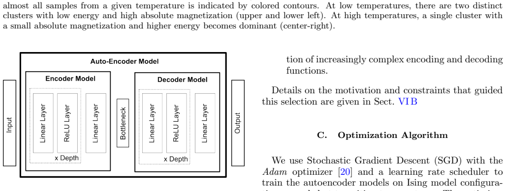
Bottleneck Size The size of the lowest-dimensional latent space, thebottleneck sizeb, can be viewed as a task choice, rather than an optimization hyperparameter. As the bottleneck size decreases, more nonlinearities are required to achieve better reconstruction performance. Th...
-
[58]
This results in a uniform block structure for both the encoder and decoder
Model Width We keep the architecture simple by using the same width for all intermediate layers except for the bottleneck. This results in a uniform block structure for both the encoder and decoder. Similar to the bottleneck, themodel widthwinfluences the degree of linear comp...
-
[59]
Theoretically, the maximum number of piecewise linear segments in a ReLU model’s function grows exponentially with the depth [52]
Model Depth The depth of a model limits its capacity to perform a sequence of operations to generate an output. Theoretically, the maximum number of piecewise linear segments in a ReLU model’s function grows exponentially with the depth [52]. In contrast, this number increases...
-
[60]
A larger batch size reduces fluctuations in the driving forces across epochs because each batch is more likely to contain similar data points
Batch Size Thebatch size|B|refers to the number of samples processed simultaneously to calculate model parameter gradients during each optimization step. A larger batch size reduces fluctuations in the driving forces across epochs because each batch is more likely to contain s...
-
[61]
Learning Rate Thelearning ratedetermines the size of the steps taken during the optimization process. This factor affects how effectively the model can avoid settling into narrow, local minima: When the parameter fluctuations are adjusted, naturally, they alter the course of t...
-
[62]
The function measures the difference between the training batch inputs,x b, and the outputs,ˆ xb
Loss Function The learning process is guided by an evaluation of the mean-squared error loss, denotedL MSD (xb,ˆ xb), which is a feature defined externally to the neural network state itself. The function measures the difference between the training batch inputs,x b, and the o...
-
[63]
Hyper-parameter Combinations Category Hyper-parameters Combi. Constants Number of steps: 100,000 Weight decay: 0.0 Dataset size: 300,000 1 Model classes Model depths: 1, 4, 16 Model widths: 256, 512, 1024 Bottleneck sizes: 1, 8, 64 27 Statistics Initialization seeds: 0, 1 Trai...
2000
-
[64]
Let’s assume a periodic error signal with period 3, resulting inL MSD k=1 = 1 2 : e=e= [1,− 1 2 ,− 1 2 ,1,− 1 2 ,− 1 2 ,
Example of non-monotonic loss scaling In the following, we provide a counterexample to prove that losses are not necessarily decreasing for larger averaging scales. Let’s assume a periodic error signal with period 3, resulting inL MSD k=1 = 1 2 : e=e= [1,− 1 2 ,− 1 2 ,1,− 1 2 ...
-
[65]
20, 21, and 22
Magnetization Exemplary loss curves showing the MSD between input and output magnetization for various learning rates are shown in Fig. 20, 21, and 22
-
[66]
Energies In contrast to magnetization, which is an order parameter and a mean variable or “field” without an inherent scale, the coarse-graining scale is a relevant variable for the energy function/operator, which is defined through local gradients in the configurations, i.e.,...
-
[67]
Principal Components All loss curves showing the MSD between input and output principal components. FIG. 24. Average validation loss evolution over training checkpoints for allMB8DXWX runs(see Tab. II) with a learning rate ofλ= 10 −4 and a bottleneck size ofb= 8. The validatio...
-
[68]
Magnetization FIG. 25. Input vs. output magnetization of all training (blue) and validation (orange) samples for different model checkpoints ofrun MB8(see Tab. II) during training. Initially, almost all outputs have the same magnetization valueM=−256. After the first 68 steps,...
-
[69]
26, we explore how the autoencoder forms an approximation for the true energy concept–by looking at the co-evolving output and input distributions of the global energy (Eq
Energy In Fig. 26, we explore how the autoencoder forms an approximation for the true energy concept–by looking at the co-evolving output and input distributions of the global energy (Eq. 2). Notably, for the bottleneck-8 system specified, around step 68, the co-distribution c...
-
[70]
Magnetization FIG. 29. Evolution of mean-square displacement (MSD) between the starting point and points along the recursion trajectories inside the 8-dimensional latent representation forrun MB8(see Tab. II) shown in Fig. 9. Each curve is colored according to the magnetizatio...
-
[71]
Energy FIG. 31. The first two principal components of the trajectory of the 8-dimensional latent representation of validation samples. The trajectory is obtained by recursively applying the autoencoder model to initial samples, and is defined by the autoencoder’s state at diff...
-
[72]
Small Bottleneck FIG. 33. Spearman rank correlation between the input magnetization difference and latent space representation distance (L2-norm) of sampled validation data pairs. The correlation is shown for different training checkpoints ofrun MB1(see Tab. II) and using the ...
-
[73]
Medium Bottleneck FIG. 35. Spearman rank correlation between the input energy difference and latent space representation distance (L2-norm) of sampled validation data pairs. The correlation is shown for different training checkpoints ofrun MB8(see Tab. II) and using the latent...
-
[74]
Large Bottleneck FIG. 36. Spearman rank correlation between the input magnetization difference and latent space representation distance (L2-norm) of sampled validation data pairs. The correlation is shown for different training checkpoints ofrun MB64(see Tab. II) and using the...
Reviewed August 2, 2026 · model on record in the stance chip above.
Discussion (0). Sign in to comment.