REVIEW 3 major objections 3 minor 82 references
Completely positive master equation for arbitrary driving and small level spacing
T0 review · 3 major / 3 minor · reviewed 2026-08-14 · deepseek-v4-flash
Pith's one-line read The paper derives a completely positive Markovian master equation that remains controlled under arbitrarily fast driving and arbitrarily small level spacing.
desk verdict A serious, largely convincing construction of a time-dependent CP master equation whose headline error bound is, as the authors admit, only proven for time-independent Hamiltonians. read the letter →
The pith
A machine-rendered reading of the paper's core claim, the machinery that carries it, and where it could break.
The reading
What carries the argument
The load-bearing object is the continuous family of Lindblad operators $A_\epsilon(t)=\sqrt{\frac{\gamma(\epsilon)}{2\pi T_a}}\int_{-T_a/2}^{T_a/2}e^{i\epsilon t_1}A(t+t_1,t)\,dt_1$, where $\gamma(\epsilon)\ge 0$ is the bath spectral density, $A(t+t_1,t)$ is the system operator in the interaction picture, and $T_a$ is the coarse-graining time. These operators convert the non-CP Redfield generator into a manifestly Lindblad-form generator $\int d\epsilon\,(A_\epsilon\rho A_\epsilon^\dagger - \tfrac{1}{2}\{A_\epsilon^\dagger A_\epsilon,\rho\})$. Complete positivity follows from the positivity of $\gamma(\epsilon)$; the time-averaging over $T_a$ replaces the rotating-wave approximation, and the neglected integration corner supplies the $O(\tau_B/(T_a\tau_{SB}))$ error that buys complete positivity. Optimizing $T_a=\sqrt{\tau_B\tau_{SB}/5}$ balances the coarse-graining error against the positivity-restoring error and yields the $\sqrt{\tau_B/\tau_{SB}}$ bound.
What would settle it
Compute or simulate the exact reduced dynamics of an explicitly solvable finite bath, such as a two-level bath or a single oscillator, under a time-dependent drive with pulses much shorter than $\tau_B$, and check whether the trace-norm error against the time-dependent CGME, Eq. (110), violates $O(\sqrt{\tau_B/\tau_{SB}}\,e^{6t/\tau_{SB}})$ at fixed small $\tau_B/\tau_{SB}$; a violation, or a proven counterexample to the claimed extension of the Section 6 bounds, would falsify the central claim.
Extended reading notes
Core claim
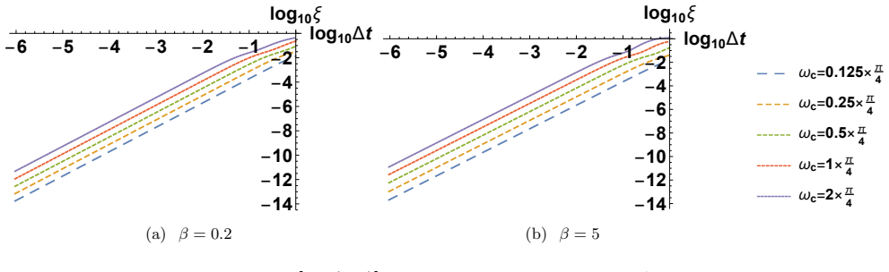
On the paper's own terms, the discovery is that the time-dependent coarse-grained master equation, Eq. (110), is a manifestly completely positive Markovian master equation valid for any time dependence of the system Hamiltonian, including instantaneous pulses. It is derived directly from the Redfield equation by coarse-graining the state over a time $T_a\sim\sqrt{\tau_B\tau_{SB}/5}$, then discarding a corner of the integration domain of area $\sim\tau_B^2$, an operation that restores complete positivity at a cost $O(\tau_B/(T_a\tau_{SB}))$. The paper claims rigorous error bounds for all three equations: Redfield, Davies-Lindblad, and CGME; the CGME bound, Eq. (28), is the only one that remains controlled as the level spacing $\delta_E$ goes to zero and as the drive becomes arbitrarily fast. The same bound is claimed for the multi-qubit generalization, with only polynomial prefactors in the system size for local observables.
Load-bearing premise
The load-bearing premise is that the rigorous error bound proved in Section 6 for a time-independent system Hamiltonian remains valid for arbitrary time-dependent driving; the authors explicitly note in footnote 5 after Eq. (28) that 'Strictly, our proof is only for the time-independent case, but there do not seem to be any obstacles for its generalization to the time-dependent case.'
Editorial extensions
If this is right
- The time-dependent CGME can describe systems driven by $\delta$-function pulses, so dynamical decoupling can be analyzed and shown to extend coherence times within a strictly Markovian setting.
- Because the Lindblad generators are spatially local when $[H,A]=O(1)$, the equation can be simulated with matrix product states or stochastic Schrödinger equations using polynomial resources, unlike the exponentially many Davies generators.
- For multi-qubit systems the error bound degrades only polynomially in system size, with a $\sqrt{n}$ or $n$ prefactor depending on noise correlations, instead of exponentially as in the Davies case.
- The bound is expressed in terms of two timescales $\tau_B$ and $\tau_{SB}$ only, so the equation's range of validity can be checked directly from the bath spectral density via $\gamma(\omega)\le 2/\tau_{SB}$ and $|\gamma'(\omega)|\le 2\tau_B/\tau_{SB}$.
- As $T_a\to\infty$ the CGME reduces to the Davies-Lindblad equation, so the Davies equation gains a controlled derivation as a limiting case rather than via the uncontrolled rotating-wave approximation.
Reading between the lines
- If the time-dependent extension of the error bound is made fully rigorous, the same coarse-graining construction may yield controlled Markovian approximations for other non-adiabatic regimes, including periodic driving beyond the Floquet-Born-Markov setup.
- The two-parameter characterization suggests a practical experimental protocol: measure the bath spectral density around the system's operating frequencies, compute $\tau_B$ and $\tau_{SB}$, and certify the CGME's range without knowing the detailed bath microphysics.
- The locality of the generators invites applying the CGME to finite-temperature many-body problems where Davies generators are nonlocal, such as energy transport or the lifetime of topologically ordered states under non-commuting couplings.
- Because the error bound is not uniform in time, a plausible next step is combining the CGME with stability or mixing arguments to obtain long-time time-independent bounds for strongly relaxing systems.
Signed reviews
Editorial analysis
A structured set of objections, weighed in public.
Referee Report
Summary. The paper derives a coarse-grained master equation (CGME) in Lindblad form, both for time-independent and time-dependent system Hamiltonians, and claims that the time-dependent CGME is completely positive, locally generated, and a controlled approximation to the true evolution for arbitrary driving and arbitrarily small level spacing. The derivation starts from the Redfield equation, introduces a coarse-graining time Ta, and shows that dropping a corner of the integration domain restores complete positivity. Error bounds are presented for Redfield, Davies-Lindblad, and CGME equations in terms of the bath timescales tau_B and tau_SB, with the CGME bound allegedly independent of the level spacing. The paper also applies the time-dependent CGME to dynamical decoupling and compares the equations numerically.
Significance. If the central claim is established, this would be a substantial advance: a completely positive Markovian master equation whose controlled error does not degrade with small level spacing and that accommodates fast, non-adiabatic driving, with immediate relevance to dynamical decoupling and gate-model quantum computing. The paper's strengths include the explicit CP construction of the CGME by corner removal, the proof that the Davies equation arises as the infinite-Ta limit, the detailed time-independent error analysis with explicit constants, and the numerical comparison with the original Redfield equation. The authors also provide reproducible code for the numerics. However, the advertised arbitrary-driving result currently rests on an unproven generalization of the time-independent error analysis, which is a load-bearing gap.
major comments (3)
- [Section 4, Eq. (110) and Eq. (28), footnote 5] The central claim that the time-dependent CGME has the controlled error (28) for arbitrary time-dependent driving is not proven. Footnote 5 after Eq. (28) states 'Strictly, our proof is only for the time-independent case', and the entire error analysis in Sec. 6 relies on the time-independent spectral decomposition A(t)=sum_omega A_omega e^{-i omega t} (Eq. (5)), the time-independent time-averaging bound (Lemma 2, Eq. (220)), and the corner-removal bound (Eq. (66)). Section 4 merely asserts after Eq. (99) that the same estimates apply, without supplying a proof for non-adiabatic H(t). In particular, the requirement that Ta be small compared with the fastest timescale of rho_I(t) cannot be satisfied when the driving is arbitrarily fast, since the driving timescale can be much shorter than any fixed Ta. This gap is load-bearing because the headline result is precisely a controlled approximation for arbitrary driving.
- [Section 6.2, Eqs. (176)-(179)] The Born approximation error is not rigorously bounded as claimed in the abstract and introduction. The text explicitly states 'we make two assumptions': that the perturbative series has a finite radius of convergence [Eq. (178)] and that the true solution is the limit of the perturbative series [Eq. (179)]. Consequently, Eq. (28) and the other error bounds are conditional on these unproven convergence assumptions. The authors should either supply a proof, cite a proof under the stated conditions, or clearly label the bounds as estimates conditional on convergence, rather than as rigorous error bounds.
- [Section 5.1, Eq. (111) and following] The dynamical decoupling application uses delta-function driving H(t)=pi/2 sum_j delta(t-j Delta t) X. For such driving U(t+t1,t) is discontinuous and H(t) is unbounded, so the error analysis used elsewhere does not directly apply. In particular, the Markov error bound in Eq. (202) uses ||dot_rho||_1 <= 4c_B/tau_SB from Eq. (40), which is derived for bounded, well-behaved A(t), and Lemma 2 also assumes a sufficiently regular generator. Section 5.1.2 computes the DD suppression factor but does not verify the error bound (28) for this case. Thus the numerical DD example does not by itself support the claim of a controlled approximation for arbitrary driving.
minor comments (3)
- [Eqs. (28), (33), (245), (249)] There are several typographical issues in the displayed equations: Eq. (28) and related places render square roots as an integral sign, and Eq. (33) has an unbalanced parenthesis. These should be corrected in production.
- [Section 4, text after Eq. (99)] The statement that the same estimates apply for the time-dependent case would benefit from at least a sketch of how the time-independent bounds generalize, and from an explicit statement of the regularity conditions on H(t) under which the generalization is expected to hold.
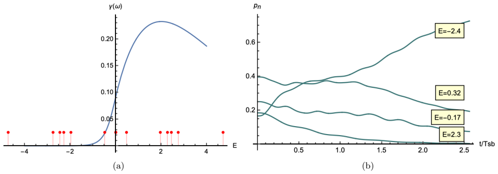
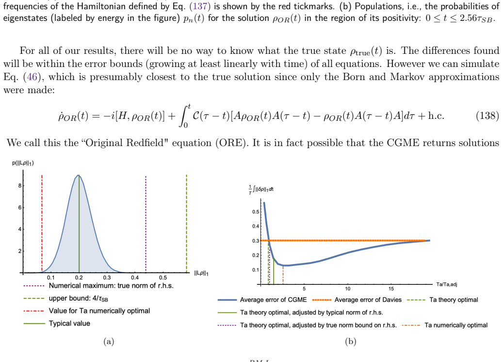
- [Section 5.3, Fig. 5] The numerical comparison with the original Redfield equation is informative, but the choice of the positivity interval for rho_OR and the use of adjusted Ta values should be described more explicitly in the figure caption so that the reader can distinguish what is fitted from what is predicted.
Circularity Check
No circularity: the CGME is rederived from the Redfield equation with explicit error bounds; the coarse-graining time is chosen by minimizing an analytic bound, not fitted to the target result.
full rationale
The derivation chain starts from the Redfield equation (42b), applies time-averaging with a free parameter Ta, and bounds each approximation error (Born, Markov, time-averaging, corner removal) in Sec. 6. The final bound Eq. (28) is obtained by optimizing the analytic expression with Ta = sqrt(tau_SB tau_B/5), so it is not a fitted input dressed as a prediction. Self-citations to [40] (original CGME) and [32] (time-averaging error analysis) are not load-bearing: Sec. 3.4 rederives the CGME from Eq. (65a), and Lemma 2 is proved in Appendix F rather than assumed. Appendix C supplies the Davies-limit proof instead of merely citing [40]. The only substantive limitation is Footnote 5 after Eq. (28): 'Strictly, our proof is only for the time-independent case, but there do not seem to be any obstacles for its generalization to the time-dependent case.' This is an explicitly admitted extension gap for the arbitrary-driving error bound, not a circular reduction; it is a correctness/verification concern outside the circularity definition. No equation in the paper is equivalent to its own input by construction, and no fitted parameter is renamed as a prediction, so the circularity score is 0.
Assumptions & free parameters
free parameters (1)
- Coarse-graining time Ta =
sqrt(tau_B tau_SB / 5) in the theoretical bound; adjusted to 1.15 Ta and 2.87 Ta in numerical examples
assumptions (5)
- domain assumption The bath state is stationary, [rho_b, H_b] = 0.
- domain assumption The bath is Gaussian, so Wick's theorem factorizes higher-order correlation functions.
- ad hoc to paper The perturbative series for the exact evolution converges, and the true solution is its limit.
- domain assumption The bath correlation time is much smaller than the fastest system decoherence timescale, tau_B << tau_SB.
- ad hoc to paper The time-independent error-bound analysis extends to arbitrary time-dependent Hamiltonians without modification.
Cite this review
Pith. "Pith review of Completely positive master equation for arbitrary driving and small level spacing." pith.science (2026). https://pith.science/paper/UL6FPG4Y
@misc{pith2026190801095,
  author       = {Pith},
  title        = {Pith review of: Completely positive master equation for arbitrary driving and small level spacing},
  year         = {2026},
  howpublished = {\url{https://pith.science/paper/UL6FPG4Y}},
  note         = {Machine review of arXiv:1908.01095}
}
read the original abstract
Markovian master equations are a ubiquitous tool in the study of open quantum systems, but deriving them from first principles involves a series of compromises. On the one hand, the Redfield equation is valid for fast environments (whose correlation function decays much faster than the system relaxation time) regardless of the relative strength of the coupling to the system Hamiltonian, but is notoriously non-completely-positive. On the other hand, the Davies equation preserves complete positivity but is valid only in the ultra-weak coupling limit and for systems with a finite level spacing, which makes it incompatible with arbitrarily fast time-dependent driving. Here we show that a recently derived Markovian coarse-grained master equation (CGME), already known to be completely positive, has a much expanded range of applicability compared to the Davies equation, and moreover, is locally generated and can be generalized to accommodate arbitrarily fast driving. This generalization, which we refer to as the time-dependent CGME, is thus suitable for the analysis of fast operations in gate-model quantum computing, such as quantum error correction and dynamical decoupling. Our derivation proceeds directly from the Redfield equation and allows us to place rigorous error bounds on all three equations: Redfield, Davies, and coarse-grained. Our main result is thus a completely positive Markovian master equation that is a controlled approximation to the true evolution for any time-dependence of the system Hamiltonian, and works for systems with arbitrarily small level spacing. We illustrate this with an analysis showing that dynamical decoupling can extend coherence times even in a strictly Markovian setting.
Figures


Figures from the paper (8 more)



Reference graph
Works this paper leans on
-
[1]
Alicki and K
R. Alicki and K. Lendi,Quantum Dynamical Semigroups and Applications(Springer Science & Business Media, 2007)
2007
-
[2]
Breuer and F
H.-P. Breuer and F. Petruccione,The Theory of Open Quantum Systems (Oxford University Press, Oxford, 2002)
2002
-
[3]
C.W. Gardiner and P. Zoller,Quantum Noise, Springer Series in Synergetics, Vol. 56 (Springer, Berlin, 2000)
work page 2000
-
[4]
E. B. Davies, “Markovian master equations,” Communications in Mathematical Physics39, 91–110 (1974)
work page 1974
-
[5]
On the generators of quantum dynamical semigroups,
G. Lindblad, “On the generators of quantum dynamical semigroups,” Comm. Math. Phys.48, 119–130 (1976)
work page 1976
-
[6]
Consistency tests of classical and quantum models for a quantum annealer,
T. Albash, W. Vinci, A. Mishra, P. A. Warburton, and D. A. Lidar, “Consistency tests of classical and quantum models for a quantum annealer,” Phys. Rev. A91, 042314– (2015)
work page 2015
-
[7]
Computational multiqubit tunnelling in programmable quantum annealers,
S. Boixo, V. N. Smelyanskiy, A. Shabani, S. V. Isakov, M. Dykman, V. S. Denchev, M. H. Amin, A. Y. Smirnov, M. Mohseni, and H. Neven, “Computational multiqubit tunnelling in programmable quantum annealers,” Nat Commun7 (2016)
work page 2016
-
[8]
Reexamination of the evidence for entanglement in a quantum annealer,
T. Albash, I. Hen, F. M. Spedalieri, and D. A. Lidar, “Reexamination of the evidence for entanglement in a quantum annealer,” Physical Review A92, 062328– (2015)
work page 2015
Show all 82 references
-
[9]
Finite temperature quantum annealing solving exponentially small gap problem with non-monotonic success probability,
A. Mishra, T. Albash, and D. A. Lidar, “Finite temperature quantum annealing solving exponentially small gap problem with non-monotonic success probability,” Nature Communications9, 2917 (2018)
2018
-
[10]
Thetheoryofageneralquantumsysteminteractingwithalineardissipative system,
R.FeynmanandF.Vernon,“Thetheoryofageneralquantumsysteminteractingwithalineardissipative system,” Annals of Physics24, 118 – 173 (1963)
1963
-
[11]
Quantum tunnelling in a dissipative system,
A. Caldeira and A. Leggett, “Quantum tunnelling in a dissipative system,” Annals of Physics149, 374 – 456 (1983)
1983
-
[12]
Path integrals for dissipative systems by tensor multiplication. condensed phase quantum dynamics for arbitrarily long time,
D. E. Makarov and N. Makri, “Path integrals for dissipative systems by tensor multiplication. condensed phase quantum dynamics for arbitrarily long time,” Chemical Physics Letters221, 482 – 491 (1994)
1994
-
[13]
Quantum dynamics for a system coupled to slow baths: On-the-fly filtered propagator method,
E. Sim, “Quantum dynamics for a system coupled to slow baths: On-the-fly filtered propagator method,” The Journal of Chemical Physics115, 4450–4456 (2001). Accepted in Quantum 2020-01-19, click title to verify. Published under CC-BY 4.0. 59
2001
-
[14]
Kraus,States, Effects, and Operations(Springer, Berlin, 1983)
K. Kraus,States, Effects, and Operations(Springer, Berlin, 1983)
1983
-
[15]
Beyond complete positivity,
J. M. Dominy and D. A. Lidar, “Beyond complete positivity,” Quant. Inf. Proc.15, 1349 (2016)
2016
-
[16]
Properties of quantum Markovian master equations,
V. Gorini, A. Frigerio, M. Verri, A. Kossakowski, and E. C. G. Sudarshan, “Properties of quantum Markovian master equations,” Reports on Mathematical Physics13, 149–173 (1978)
1978
-
[17]
On Quantum Theory of Transport Phenomena : Steady Diffusion,
S. Nakajima, “On Quantum Theory of Transport Phenomena : Steady Diffusion,” Prog. Theor. Phys. 20, 948 (1958)
1958
-
[18]
Ensemble Method in the Theory of Irreversibility,
R. Zwanzig, “Ensemble Method in the Theory of Irreversibility,” J. Chem. Phys.33, 1338 (1960)
1960
-
[19]
The theory of relaxation processes,
A. Redfield, “The theory of relaxation processes,” inAdvances in Magnetic Resonance, Advances in Magnetic and Optical Resonance, Vol. 1, edited by J. S. Waugh (Academic Press, 1965) pp. 1 – 32
1965
-
[20]
Robustness of decoherence-free subspaces for quantum computation,
D. Bacon, D. A. Lidar, and K. B. Whaley, “Robustness of decoherence-free subspaces for quantum computation,” Phys. Rev. A60, 1944–1955 (1999)
1999
-
[21]
Virtues and limitations of markovian master equations with a time-dependent generator,
A. J. van Wonderen and K. Lendi, “Virtues and limitations of markovian master equations with a time-dependent generator,” J. Stat. Phys.100, 633–658 (2000)
2000
-
[22]
From completely positive maps to the quantum Markovian semigroup master equation,
D. A. Lidar, Z. Bihary, and K. Whaley, “From completely positive maps to the quantum Markovian semigroup master equation,” Chem. Phys.268, 35 (2001)
2001
-
[23]
Depolarizing channel as a completely positive map with memory,
S. Daffer, K. Wodkiewicz, J.D. Cresser, J.K. McIver, “Depolarizing channel as a completely positive map with memory,” Phys. Rev. A70, 010304(R) (2004)
2004
-
[24]
Completely positive post-markovian master equation via a measurement approach,
A. Shabani and D. A. Lidar, “Completely positive post-markovian master equation via a measurement approach,” Phys. Rev. A71, 020101(R) (2005)
2005
-
[25]
Non-Markovian dynamics of a qubit,
S. Maniscalco and F. Petruccione, “Non-Markovian dynamics of a qubit,” Phys. Rev. A73, 012111 (2006)
2006
-
[26]
Non-markovian quantum jumps,
J. Piilo, S. Maniscalco, K. Härkönen, and K.-A. Suominen, “Non-markovian quantum jumps,” Physical Review Letters 100, 180402– (2008)
2008
-
[27]
Quantum semi-markov processes,
H.-P. Breuer and B. Vacchini, “Quantum semi-markov processes,” Physical Review Letters101, 140402– (2008)
2008
-
[28]
Staying positive: going beyond lindblad with perturbative master equations,
R. S. Whitney, “Staying positive: going beyond lindblad with perturbative master equations,” Journal of Physics A: Mathematical and Theoretical41, 175304 (2008)
2008
-
[29]
Master equation and control of an open quantum system with leakage,
L.-A. Wu, G. Kurizki, and P. Brumer, “Master equation and control of an open quantum system with leakage,” Physical Review Letters102, 080405– (2009)
2009
-
[30]
Non-markovian quantum dynamics: Local versus nonlocal,
D. Chruściński and A. Kossakowski, “Non-markovian quantum dynamics: Local versus nonlocal,” Phys. Rev. Lett. 104, 070406 (2010)
2010
-
[31]
Quantum adiabatic Markovian master equations,
T. Albash, S. Boixo, D. A. Lidar, and P. Zanardi, “Quantum adiabatic Markovian master equations,” New J. of Phys.14, 123016 (2012)
2012
-
[32]
Local master equation for small temperatures,
E. Mozgunov, “Local master equation for small temperatures,” arXiv:1611.04188 (2016)
2016 arXiv
-
[33]
Theory of open quantum dynamics with hybrid noise,
A. Y. Smirnov and M. H. Amin, “Theory of open quantum dynamics with hybrid noise,” New Journal of Physics 20, 103037 (2018)
2018
-
[34]
Time-dependent markovian quantum master equation,
R. Dann, A. Levy, and R. Kosloff, “Time-dependent markovian quantum master equation,” Phys. Rev. A 98, 052129 (2018)
2018
-
[35]
Error reduction in quantum annealing using boundary cancellation: Only the end matters,
L. C. Venuti and D. A. Lidar, “Error reduction in quantum annealing using boundary cancellation: Only the end matters,” Phys. Rev. A98, 022315 (2018)
2018
-
[36]
Completely positive, accurate master equation for weakly-damped quantum systems across all regimes,
G. McCauley, B. Cruikshank, D. I. Bondar, and K. Jacobs, “Completely positive, accurate master equation for weakly-damped quantum systems across all regimes,” arXiv:1906.08279 (2019)
2019 arXiv
-
[37]
Environment-induced entanglement in a refined weak- coupling limit,
F. Benatti, R. Floreanini, and U. Marzolino, “Environment-induced entanglement in a refined weak- coupling limit,” EPL (Europhysics Letters)88, 20011 (2009)
2009
-
[38]
Entangling two unequal atoms through a common bath,
F. Benatti, R. Floreanini, and U. Marzolino, “Entangling two unequal atoms through a common bath,” Phys. Rev. A81, 012105 (2010)
2010
-
[39]
Quantum markovian master equations: Resonance theory shows validity for all time scales,
M. Merkli, “Quantum markovian master equations: Resonance theory shows validity for all time scales,” Annals of Physics412, 167996 (2020)
2020
-
[40]
Coarse graining can beat the rotating-wave approximation in quantum markovian master equations,
C. Majenz, T. Albash, H.-P. Breuer, and D. A. Lidar, “Coarse graining can beat the rotating-wave approximation in quantum markovian master equations,” Phys. Rev. A88, 012103– (2013)
2013
-
[41]
Stability of local quantum dissipative systems,
T. S. Cubitt, A. Lucia, S. Michalakis, and D. Perez-Garcia, “Stability of local quantum dissipative systems,” Communications in Mathematical Physics337, 1275–1315 (2015)
2015
-
[42]
Quantum computing with realistically noisy devices,
E. Knill, “Quantum computing with realistically noisy devices,” Nature434, 39–44 (2005). Accepted in Quantum 2020-01-19, click title to verify. Published under CC-BY 4.0. 60
2005
-
[43]
Internal consistency of fault-tolerant quantum error correction in light of rigorous derivations of the quantum markovian limit,
R. Alicki, D. A. Lidar, and P. Zanardi, “Internal consistency of fault-tolerant quantum error correction in light of rigorous derivations of the quantum markovian limit,” Phys. Rev. A73, 052311 (2006)
2006
-
[44]
Lecture notes on the theory of open quantum systems,
D. A. Lidar, “Lecture notes on the theory of open quantum systems,” arXiv preprint arXiv:1902.00967 (2019)
2019 arXiv
-
[45]
Decoherence in adiabatic quantum computation,
T. Albash and D. A. Lidar, “Decoherence in adiabatic quantum computation,” Phys. Rev. A91, 062320– (2015)
2015
-
[46]
Dephasing-induced diffusive transport in the anisotropic heisenberg model,
M. Žnidarič, “Dephasing-induced diffusive transport in the anisotropic heisenberg model,” New Journal of Physics 12, 043001 (2010)
2010
-
[47]
Influence of dephasing on many-body localization,
M. V. Medvedyeva, T. Prosen, and M. Žnidarič, “Influence of dephasing on many-body localization,” Phys. Rev. B93, 094205 (2016)
2016
-
[48]
Bhatia,Matrix Analysis, Graduate Texts in Mathematics No
R. Bhatia,Matrix Analysis, Graduate Texts in Mathematics No. 169 (Springer-Verlag, New York, 1997)
1997
-
[49]
Slippage of initial conditions for the redfield master equation,
P. Gaspard and M. Nagaoka, “Slippage of initial conditions for the redfield master equation,” Journal of Chemical Physics 111, 5668–5675 (1999)
1999
-
[50]
Efficient classical simulation of slightly entangled quantum computations,
G. Vidal, “Efficient classical simulation of slightly entangled quantum computations,” Phys. Rev. Lett. 91, 147902 (2003)
2003
-
[51]
Matrix product density operators: Simulation of finite-temperature and dissipative systems,
F. Verstraete, J. J. Garcia-Ripoll, and J. I. Cirac, “Matrix product density operators: Simulation of finite-temperature and dissipative systems,” Phys. Rev. Lett.93, 207204 (2004)
2004
-
[52]
The finite group velocity of quantum spin systems,
E. H. Lieb and D.W. Robinson, “The finite group velocity of quantum spin systems,” Commun. Math. Phys. 28, 251 (1972)
1972
-
[53]
Quantumalgorithmforsimulatingrealtimeevolution of lattice hamiltonians,
J.Haah, M.Hastings, R.Kothari, andG.H.Low,“Quantumalgorithmforsimulatingrealtimeevolution of lattice hamiltonians,” in2018 IEEE 59th Annual Symposium on Foundations of Computer Science (FOCS) (2018) pp. 350–360
2018
-
[54]
Nonequilibrium dynamics of bosonic atoms in optical lattices: Decoherence of many-body states due to spontaneous emission,
H. Pichler, A. J. Daley, and P. Zoller, “Nonequilibrium dynamics of bosonic atoms in optical lattices: Decoherence of many-body states due to spontaneous emission,” Phys. Rev. A82, 063605 (2010)
2010
-
[55]
Reducing decoherence in quantum-computer memory with all quantum bits coupling to the same environment,
L.-M Duan and G.-C. Guo, “Reducing decoherence in quantum-computer memory with all quantum bits coupling to the same environment,” Phys. Rev. A57, 737 (1998)
1998
-
[56]
Noiseless quantum codes,
P. Zanardi and M. Rasetti, “Noiseless quantum codes,” Phys. Rev. Lett.79, 3306–3309 (1997)
1997
-
[57]
Decoherence-free subspaces for quantum computation,
D. A. Lidar, I. L. Chuang, and K. B. Whaley, “Decoherence-free subspaces for quantum computation,” Phys. Rev. Lett.81, 2594–2597 (1998)
1998
-
[58]
Decoherence-free subspaces and subsystems,
D. A. Lidar and K. B. Whaley, “Decoherence-free subspaces and subsystems,” inIrreversible Quantum Dynamics, Lecture Notes in Physics, Vol. 622, edited by F. Benatti and R. Floreanini (Springer, Berlin,
-
[59]
Experimental Verification of Decoherence- Free Subspaces,
P.G. Kwiat, A.J. Berglund, J.B. Altepeter, and A.G. White, “Experimental Verification of Decoherence- Free Subspaces,” Science290, 498 (2000)
2000
-
[60]
Experimental realization of noiseless subsystems for quantum information processing,
L. Viola, E. M. Fortunato, M. A. Pravia, E. Knill, R. Laflamme, and D. G. Cory, “Experimental realization of noiseless subsystems for quantum information processing,” Science293, 2059–2063 (2001)
2001
-
[61]
A decoherence-free quantum memory using trapped ions,
D. Kielpinski, V. Meyer, M. A. Rowe, C. A. Sackett, W. M. Itano, C. Monroe, and D. J. Wineland, “A decoherence-free quantum memory using trapped ions,” Science291, 1013–1015 (2001)
2001
-
[62]
Magnetic resonance realization of decoherence-free quantum computation,
J. E. Ollerenshaw, D. A. Lidar, and L. E. Kay, “Magnetic resonance realization of decoherence-free quantum computation,” Phys. Rev. Lett.91, 217904 (2003)
2003
-
[63]
Dynamical suppression of decoherence in two-state quantum systems,
L. Viola and S. Lloyd, “Dynamical suppression of decoherence in two-state quantum systems,” Phys. Rev. A 58, 2733–2744 (1998)
1998
-
[64]
Symmetrizing evolutions,
P. Zanardi, “Symmetrizing evolutions,” Physics Letters A258, 77–82 (1999)
1999
-
[65]
Lidar and T
D. Lidar and T. Brun, eds.,Quantum Error Correction(Cambridge University Press, Cambridge, UK, 2013)
2013
-
[66]
Colloquium: Protectingquantuminformationagainstenvironmentalnoise,
D.SuterandG.A.Álvarez,“Colloquium: Protectingquantuminformationagainstenvironmentalnoise,” Reviews of Modern Physics88, 041001– (2016)
2016
-
[67]
Combining dynamical decoupling with fault-tolerant quantum computation,
H. K. Ng, D. A. Lidar, and J. Preskill, “Combining dynamical decoupling with fault-tolerant quantum computation,” Phys. Rev. A84, 012305– (2011)
2011
-
[68]
Markovian theory of dynamical decoupling by periodic control,
K. Szczygielski and R. Alicki, “Markovian theory of dynamical decoupling by periodic control,” Physical Review A 92, 022349– (2015)
2015
-
[69]
Can quantum markov evolutions ever be dynamically decoupled?
J. E. Gough and H. I. Nurdin, “Can quantum markov evolutions ever be dynamically decoupled?” in 2017 IEEE 56th Annual Conference on Decision and Control (CDC)(2017) pp. 6155–6160. Accepted in Quantum 2020-01-19, click title to verify. Published under CC-BY 4.0. 61
2017
-
[70]
Dynamical decoupling efficiency versus quantum non-markovianity,
C. Addis, F. Ciccarello, M. Cascio, G. M. Palma, and S. Maniscalco, “Dynamical decoupling efficiency versus quantum non-markovianity,” New Journal of Physics17, 123004 (2015)
2015
-
[71]
Dynamical decoupling of unbounded hamiltonians,
C. Arenz, D. Burgarth, P. Facchi, and R. Hillier, “Dynamical decoupling of unbounded hamiltonians,” Journal of Mathematical Physics, Journal of Mathematical Physics59, 032203 (2018)
2018
-
[72]
Concepts of quantum non-markovianity: A hierarchy,
L. Li, M. J. W. Hall, and H. M. Wiseman, “Concepts of quantum non-markovianity: A hierarchy,” Concepts of quantum non-Markovianity: A hierarchy, Physics Reports759, 1–51 (2018)
2018
-
[73]
Effects of dissipation on an adiabatic quantum search algo- rithm,
I. de Vega, M. C. Bañuls, and A. Pérez, “Effects of dissipation on an adiabatic quantum search algo- rithm,” New J. of Phys.12, 123010 (2010)
2010
-
[74]
https://github.com/mvjenia/CGMEcode, code for the numerical section of the paper
-
[75]
On certain probable errors and correlation coefficients of multiple frequency distributions with skew regression,
L. Isserlis, “On certain probable errors and correlation coefficients of multiple frequency distributions with skew regression,” Biometrika11, 185 (1916)
1916
-
[76]
Fluctuation theorems for quantum processes,
T. Albash, D. A. Lidar, M. Marvian, and P. Zanardi, “Fluctuation theorems for quantum processes,” Phys. Rev. E88, 032146– (2013)
2013
-
[77]
Adiabatic quantum computation,
T. Albash and D. A. Lidar, “Adiabatic quantum computation,” Reviews of Modern Physics90, 015002– (2018)
2018
-
[78]
A statistical mechanics view on kitaev’s proposal for quantum memories,
R. Alicki, M. Fannes, and M. Horodecki, “A statistical mechanics view on kitaev’s proposal for quantum memories,” Journal of Physics A: Mathematical and Theoretical40, 6451–6467 (2007)
2007
-
[79]
Topological subsystem codes,
H. Bombin, “Topological subsystem codes,” Physical Review A81, 032301– (2010)
2010
-
[80]
Anderson localization makes adiabatic quantum optimization fail,
B. Altshuler, H. Krovi, and J. Roland, “Anderson localization makes adiabatic quantum optimization fail,” Proceedings of the National Academy of Sciences107, 12446–12450 (2010)
2010
-
[81]
Reed and B
M. Reed and B. Simon,Methods of Modern Mathematical Physics: Fourier analysis, self-adjointness, Vol. 2 (Academic Press, 1975)
1975
-
[82]
On some inequalities for the incomplete gamma function,
H. Alzer, “On some inequalities for the incomplete gamma function,” Mathematics of Computation66, 771 (1997). Accepted in Quantum 2020-01-19, click title to verify. Published under CC-BY 4.0. 62
1997
Reviewed August 14, 2026 · model on record in the stance chip above.
Discussion (0). Continue with ORCID to comment.