REVIEW 3 major objections 5 minor 46 references
Replacing high-noise nodes with classical simulations can make zero-noise extrapolation's sampling variance fall exponentially in the Richardson order.
Reviewed by Pith at T0; open to challenge. T0 means a machine referee read the full paper against a public rubric. the ladder, T0–T4 →
T0 review · deepseek-v4-flash
2026-08-01 01:34 UTC pith:UM4ZCCJW
load-bearing objection The variance-reduction formula is correct and verified, but the exponential claim is coefficient-level only; the missing scaling analysis of the bias term means the practical MSE advantage at large n is unestablished. the 3 major comments →
Classically Augmented Zero-Noise Extrapolation
The pith
A machine-rendered reading of the paper's core claim, the machinery that carries it, and where it could break.
Core claim
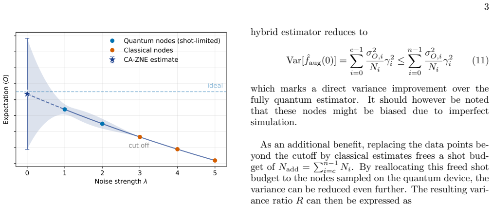
On its own terms, the central claim is that CA-ZNE reallocates the sampling-variance bottleneck of ZNE into a controlled classical-bias budget: the variance ratio between CA-ZNE and standard ZNE, under optimal shot allocation and equal per-node observable variances, is R = (Σ_{j=0}^{c-1}|γ_j| / Σ_{i=0}^{n-1}|γ_i|)^2, where the γ are Richardson interpolation weights and c is the number of quantum nodes. Because the weights for linear node spacing x_j = 1 + j are binomial, |γ_j| = binom(n, j+1), the denominator is 2^n − 1 while the numerator grows only polynomially for fixed c, so R decays exponentially in n. The paper further shows that the bias of the augmented estimator decomposes into the
What carries the argument
The central object is the Richardson-extrapolation weight set {γ_i}, the Lagrange coefficients that map noisy expectation values at amplified noise levels to the zero-noise estimate. CA-ZNE's mechanism is to zero out the sampling contribution of the high-noise nodes by replacing them with deterministic classical estimates, then redistribute the freed shot budget among the remaining quantum nodes; the identity carrying the argument is the variance-reduction ratio R = (Σ_{j<c}|γ_j| / Σ_{i<n}|γ_i|)^2. For linear spacing the weights become binomial coefficients, which turns the calculation of R into a binomial-identity problem and yields the exponential reduction. The companion piece is the bias
Load-bearing premise
The classical estimates at the replaced high-noise nodes must be accurate enough—after being multiplied by the same Richardson weights—that the bias they add does not outweigh the variance they remove; the paper's demonstrations use only modest extrapolation orders and do not analyze how the bias bound scales as the order grows.
What would settle it
Compute the mean-squared error of CA-ZNE versus standard ZNE for a fixed observable as the Richardson order n increases at a fixed classical truncation budget. The coefficient-level formula predicts R ~ (binom(n,c)/(2^n−1))^2, an exponential variance reduction; but if the measured MSE stops improving or worsens because the weighted truncation-bias term Σ_{i≥c} binom(n,i+1) e^{−ν x_i(l+1)} does not decay with n (which it cannot for bounded linear spacing and fixed l), then the practical advantage claimed for large n fails even though the coefficient-level ratio is correct.
If this is right
- For linearly spaced noise levels, CA-ZNE can convert ZNE's exponential sampling overhead into exponential variance reduction at fixed cutoff, making linear spacing competitive with Chebyshev spacings in sampling cost.
- The coefficient-level variance reduction is circuit-independent and depends only on node spacing and cutoff, so the same formula applies across circuits; circuit dependence enters through the attainable classical bias and cutoff location.
- CA-ZNE improves MSE only when the weighted classical truncation bias is smaller than the variance it eliminates; increasing the classical truncation budget is the practical lever for reaching this regime.
- For Chebyshev-type node spacings the variance reduction is more modest but still practically relevant, reaching one to four orders of magnitude for Chebyshev roots at higher orders.
- The method creates a concrete division of labor: quantum hardware is needed for the low-noise nodes where high-weight Pauli signals remain visible, while high-noise nodes, where such signals are exponentially suppressed, can be delegated to classical simulation.
Where Pith is reading between the lines
- A necessary follow-up is a scaling analysis of the bias term: with a fixed classical truncation threshold, the bias contribution weighted by the Richardson coefficients can grow like 2^n for bounded linear spacing, so the exponential variance reduction may not translate to exponential MSE reduction at large n unless the truncation threshold grows with n.
- The same logic suggests a sharp criterion for when CA-ZNE is useful: observables dominated by low-weight Pauli terms at high noise will be classically simulable there, while observables with significant high-weight contributions will produce large simulation bias; this can be tested by varying the Pauli-weight distribution of the observable.
- The freed shot budget need not simply reduce variance; it could be redirected to more sophisticated mitigation at the remaining quantum nodes, such as partial probabilistic error cancellation, an extension the paper names as promising.
- The result also implies that the node spacings optimal for standard ZNE are not necessarily optimal for CA-ZNE; spacing optimization in the augmented setting is a natural extension.
Editorial analysis
A structured set of objections, weighed in public.
Referee Report
Summary. The paper proposes Classically Augmented Zero-Noise Extrapolation (CA-ZNE), in which the high-noise nodes of a Richardson extrapolation are replaced by deterministic classical estimates obtained from truncated Pauli propagation. Under optimal shot allocation and equal per-node variances, the variance of the augmented estimator relative to standard ZNE is shown to be R = (Σ_{j<c}|γ_j| / Σ_{i<n}|γ_i|)^2 (Eq. 13). For linear node spacings the interpolation weights are binomially distributed, so for fixed cutoff c the ratio R decays exponentially in the Richardson order n (Appendix C). The variance-reduction formula is validated numerically on a transverse-field Ising model (analytic R=0.444 versus measured R=0.445) and on a Schwinger-model benchmark, and MSE improvements are demonstrated when the classical truncation bias is small. The paper is careful to call the exponential reduction 'coefficient-level' in the abstract and to warn that the method reallocates variance into classical bias.
Significance. If the end-to-end advantage held, CA-ZNE would be a practically valuable method for reducing the sampling overhead of ZNE, especially for linear node spacings where ordinary ZNE overhead grows exponentially. The derivation of the variance-reduction ratio is clean, the Monte Carlo check is convincing, and the numerical experiments support the coefficient-level claims. The paper also makes a useful conceptual point: node spacings optimized for standard ZNE need not remain optimal when zero-variance classical anchor points are available. The central gap is that the exponential variance reduction is only a coefficient-level statement; the bias bound that controls the actual MSE is not shown to remain small as the Richardson order grows. Because the paper's practical promise depends on this bias-variance tradeoff, the current evidence is not sufficient for the full claim as stated.
major comments (3)
- [Sec. III C, Eq. (23); Sec. IV.D] The bias term in Eq. (23) is not analyzed under the linear spacing actually used in the scaling study. For linear nodes on [1,B], the weights satisfy |γ_i| ∝ binom(n-1,i)/(1+h i) (see Appendix C), so Σ_{i=c}^{n-1}|γ_i| grows like 2^n. Since all x_i ≥ 1, the simulation-bias term in Eq. (23) is at most √(d+1)||O||_F e^{-ν_eff(l+1)} Σ_{i=c}^{n-1}|γ_i|, which for fixed truncation threshold l grows exponentially with n. Thus the same Richardson weights that produce the exponential variance reduction also multiply the classical bias, and the paper does not provide a scaling analysis showing how l (or another truncation parameter) must grow with n to keep the squared bias below the variance. The numerical demonstrations use only n=4 or 5 nodes, and Figs. 7 and 8 plot R and Λ² only, not MSE or classical cost. This is load-bearing for the practical claim that CA-ZNE 'can be exponential' as an end
- [Sec. IV.A and IV.B; Fig. 5] The numerical truncation is performed with Qiskit's max_terms parameter, which the paper states is not identical to the weight threshold l appearing in Eqs. (22)-(23). The theoretical bound is therefore used only as motivation, and the empirical bias curves in Fig. 5 are not connected quantitatively to the bound. Consequently the required condition 'when the truncation bias is sufficiently small' is not tied to a controllable parameter in a way that would let a user predict when CA-ZNE will improve over ZNE. Please provide either a quantitative mapping from max_terms (or an analogous resource parameter) to the bias bound, or an empirical scaling law that can be used as a cutoff-selection criterion.
- [Sec. VI; Sec. V] The conclusion states that 'the classical estimates must become increasingly accurate as more nodes ... are offloaded,' and Sec. V notes that the required Pauli-propagation run-times can be 'impractical despite being formally quasi-polynomial.' These admissions correctly identify the bias-variance-cost tradeoff, but they also highlight that the paper does not quantify it. The abstract's qualifier 'coefficient-level' is appropriate, but the introduction and conclusion present the reduction as a practical advantage ('reduction in sampling overhead can reach several orders of magnitude in favorable regimes'). To support the stronger reading, the paper needs an end-to-end MSE analysis that includes the bias and classical cost as functions of n, c, and the truncation threshold, not only the variance ratio.
minor comments (5)
- [Abstract/Title] The spelling is inconsistent: 'Classically Augmented' in the title and abstract but 'Classically-Augmented' in the section heading. Please unify.
- [Eq. (7) and surrounding text] The symbol σ_{O,i} is used before being defined; define it explicitly when the per-node variances are introduced.
- [Sec. III C, Eq. (23)] In Eq. (23) the bias is written as Bias[\hat f_aug] but the bound is on the absolute expectation; clearer notation would be |E[\hat f_aug]-⟨O⟩_0|. Also define δ_i before Eq. (B3).
- [Fig. 6] Figure 6 contains corrupted glyphs (e.g., '/uni00000013...'), suggesting a font-embedding problem. Please regenerate the figure.
- [Data availability] The statement 'All data ... available from the author upon reasonable request' is weaker than the reproducibility standard typical for this field. Consider releasing the simulation scripts and data.
Circularity Check
No significant circularity: the variance-reduction ratio is derived algebraically from definitions and independent interpolation-weight identities, validated by Monte Carlo, with all load-bearing bias and simulation bounds imported from external sources.
full rationale
The central derivation is self-contained. Equation (13) follows from Eq. (9)'s optimal shot allocation and Eq. (11)'s zero-variance classical-node assumption: with N_i proportional to |γ_i| over the c quantum nodes, the variance is (Σ_{j<c}|γ_j|)^2 σ²/N_shots, so the ratio to standard ZNE is the square of the coefficient-sum ratio. This is a direct algebraic identity, not a fit. Appendix C's exponential scaling uses the standard identity for linear spacing |γ_j| = binom(n, j+1) (Eq. C4), credited to external Ref. [23], and the binomial theorem (C6); the Monte Carlo check (R = 0.445 measured vs 0.444 analytic) is an independent numerical confirmation, not an input to the derivation. The bias bound Eq. (23) and the Pauli-propagation algorithm are imported from external Ref. [30] with stated assumptions, and Appendix A derives the SPL-to-depolarizing bound from definitions. The only self-citation, Ref. [24], appears in a related-work list and is not load-bearing. The paper's own caveats (Secs V and VI: classical estimates must become increasingly accurate; some runtimes may be impractical) flag a practical bias/resource limitation, but they do not make any derived prediction an input. Therefore no circularity is present.
Axiom & Free-Parameter Ledger
free parameters (3)
- cutoff index c =
2-3 in experiments; varied in scaling study
- Pauli-propagation truncation budget (max_terms / weight cutoff l) =
10^2 to 10^5 retained Pauli terms
- node spacing parameters (step h, interval bound B, Chebyshev x_1) =
B=5 in scaling study, [1,3] in Schwinger model, linear step h chosen to cover interval
axioms (8)
- standard math The noisy expectation-value curve g(x)=⟨O⟩_{λ0 x} is n-times differentiable and the standard polynomial interpolation error formula applies.
- domain assumption Per-node sampling variances are equal: σ_{O,i}=σ_O.
- domain assumption Sampling estimates across different noise nodes are statistically independent.
- domain assumption The classical simulator is deterministic with negligible numerical variance, so its only error is the bias δ_i.
- domain assumption The classical bias bound of Ref [30] holds: |δ_i| ≤ e^{-ν_i(l+1)}√(d+1)||O||_F in root-mean-square over an ensemble of input states.
- domain assumption The SPL noise model sufficiently approximates the device noise; noise-model mismatch is neglected.
- ad hoc to paper The numerical Pauli-propagation truncation (max_terms) behaves like the weight cutoff l in the theoretical bound.
- domain assumption The amplified noise levels remain below the signal-retaining floor of Ref [39].
read the original abstract
We investigate a hybrid quantum-classical approach to quantum error mitigation. We propose Classically Augmented Zero-Noise Extrapolation, a hybrid error-mitigation method in which high-noise Richardson extrapolation nodes are replaced by classically simulated estimates. These classical nodes have negligible sampling variance but introduce deterministic simulation bias. We derive the resulting variance reduction under optimal shot allocation and show that, for linear node spacings and fixed index cutoff, the coefficient-level reduction can be exponential. We validate the prediction numerically using Pauli-propagation simulations and demonstrate a reduction in mean-squared error when the truncation bias is sufficiently small.
Figures


Reference graph
Works this paper leans on
-
[1]
The SPL channel is diagonal in the Pauli basis, so each Pauli operatorPis an eigenoperator ofNwith eigenvalue (cf
Interaction with SPL noise Pauli propagation is particularly well suited for simu- lating the SPL noise model because of its simple action on Pauli observables. The SPL channel is diagonal in the Pauli basis, so each Pauli operatorPis an eigenoperator ofNwith eigenvalue (cf. Eq. (18)) N(P) =e −2 P k∈K λk⟨P,Pk⟩ P,(30) where⟨P, P k⟩denotes the symplectic in...
-
[2]
Bauer, S
B. Bauer, S. Bravyi, M. Motta, and G. K.-L. Chan, Chemical Reviews120, 12685 (2020)
2020
-
[3]
Babbush, R
R. Babbush, R. King, S. Boixo, W. Huggins, T. Khattar, G. H. Low, J. R. McClean, T. O’Brien, and N. C. Rubin, PRX Quantum7, 020101 (2026)
2026
-
[4]
Santagati, A
R. Santagati, A. Aspuru-Guzik, R. Babbush, M. Deg- roote, L. Gonz´ alez, E. Kyoseva, N. Moll, M. Oppel, R. M. Parrish, N. C. Rubin,et al., Nature Physics20, 549 (2024)
2024
-
[5]
Bluvstein, S
D. Bluvstein, S. J. Evered, A. A. Geim, S. H. Li, H. Zhou, T. Manovitz, S. Ebadi, M. Cain, M. Kalinowski, D. Hangleiter, J. P. Bonilla Ataides,et al., Nature626, 58 (2024)
2024
-
[6]
Morvan, B
A. Morvan, B. Villalonga, X. Mi, S. Mandr` a, A. Bengts- son, P. Klimov, Z. Chen, S. Hong, C. Erickson, I. Droz- dov,et al., Nature634, 328 (2024)
2024
-
[7]
Mazurenko, C
A. Mazurenko, C. S. Chiu, G. Ji, M. F. Parsons, M. Kan´ asz-Nagy, R. Schmidt, F. Grusdt, E. Demler, D. Greif, and M. Greiner, Nature545, 462 (2017)
2017
-
[8]
Y. Kim, A. Eddins, S. Anand, K. X. Wei, E. Van Den Berg, S. Rosenblatt, H. Nayfeh, Y. Wu, M. Zale- tel, K. Temme,et al., Nature618, 500 (2023)
2023
-
[9]
Tindall, M
J. Tindall, M. Fishman, E. M. Stoudenmire, and D. Sels, PRX Quantum5, 010308 (2024)
2024
-
[10]
M. S. Rudolph, E. Fontana, Z. Holmes, and L. Cincio, arXiv preprint arXiv:2308.09109 (2023), 10.48550/arXiv.2308.09109
-
[11]
Yamamoto, Y
K. Yamamoto, Y. Kikuchi, D. Amaro, B. Criger, S. Dilkes, C. Ryan-Anderson, A. Tranter, J. M. Dreil- ing, D. Gresh, C. Foltz,et al., PRX Quantum7, 020319 (2026)
2026
-
[12]
Z. Cai, R. Babbush, S. C. Benjamin, S. Endo, W. J. Hug- gins, Y. Li, J. R. McClean, and T. E. O’Brien, Reviews of Modern Physics95, 045005 (2023)
2023
-
[13]
Temme, S
K. Temme, S. Bravyi, and J. M. Gambetta, Physical review letters119, 180509 (2017)
2017
-
[14]
Van Den Berg, Z
E. Van Den Berg, Z. K. Minev, A. Kandala, and K. Temme, Nature physics19, 1116 (2023)
2023
-
[15]
Czarnik, A
P. Czarnik, A. Arrasmith, P. J. Coles, and L. Cincio, Quantum5, 592 (2021)
2021
-
[16]
W. J. Huggins, S. McArdle, T. E. O’Brien, J. Lee, N. C. Rubin, S. Boixo, K. B. Whaley, R. Babbush, and J. R. McClean, Physical Review X11, 041036 (2021)
2021
-
[17]
Koczor, Physical Review X11, 031057 (2021)
B. Koczor, Physical Review X11, 031057 (2021)
2021
-
[18]
S. Endo, S. C. Benjamin, and Y. Li, Phys. Rev. X8, 031027 (2018)
2018
-
[19]
Kandala, K
A. Kandala, K. Temme, A. D. C´ orcoles, A. Mezzacapo, J. M. Chow, and J. M. Gambetta, Nature567, 491 (2019)
2019
-
[20]
Li and S
Y. Li and S. C. Benjamin, Physical Review X7, 021050 12 (2017)
2017
-
[21]
Giurgica-Tiron, Y
T. Giurgica-Tiron, Y. Hindy, R. LaRose, A. Mari, and W. J. Zeng, in2020 IEEE international conference on quantum computing and engineering (QCE)(IEEE,
-
[22]
Majumdar, P
R. Majumdar, P. Rivero, F. Metz, A. Hasan, and D. S. Wang, in2023 IEEE International Conference on Quan- tum Computing and Engineering (QCE), Vol. 1 (IEEE,
-
[23]
A. He, B. Nachman, W. A. de Jong, and C. W. Bauer, Physical Review A102, 012426 (2020)
2020
-
[24]
Mohammadipour and X
P. Mohammadipour and X. Li, Quantum9, 1909 (2025)
1909
-
[25]
Scheiber, P
T. Scheiber, P. Haubenwallner, and M. Heller, Quantum 9, 1840 (2025)
2025
-
[26]
S. Filippov, M. Leahy, M. A. Rossi, and G. Garc ´ ıa- P´ erez, arXiv preprint arXiv:2307.11740 (2023), 10.48550/arXiv.2307.11740
-
[27]
S. Majumder, J. Garrison, L. Luo, B. Mitchell, M. Amico, A. Seif, M. Tran, K. Sharma, E. Berg, Z. Minev,et al., arXiv preprint arXiv:2603.14485 (2026), 10.48550/arXiv.2603.14485
-
[28]
Krebsbach, B
M. Krebsbach, B. Trauzettel, and A. Calzona, Physical Review A106, 062436 (2022)
2022
-
[29]
Cai, arXiv preprint arXiv:2110.05389 (2021), https://doi.org/10.48550/arXiv.2110.05389
Z. Cai, arXiv preprint arXiv:2110.05389 (2021), https://doi.org/10.48550/arXiv.2110.05389
-
[30]
Angrisani, A
A. Angrisani, A. A. Mele, M. S. Rudolph, M. Cerezo, and Z. Holmes, PRX Quantum7, 020313 (2026)
2026
-
[31]
Schuster, C
T. Schuster, C. Yin, X. Gao, and N. Y. Yao, Physical Review X15, 041018 (2025)
2025
-
[32]
Malekakhlagh, A
M. Malekakhlagh, A. Seif, D. Puzzuoli, L. C. Govia, and E. van den Berg, npj Quantum Information11, 191 (2025)
2025
-
[33]
Better Pauli Channel Learning with Maximum Likelihood Estimation
D. Belkin, F. Alam, M. Thibodeau, A. Seif, E. v. d. Berg, and B. K. Clark, arXiv preprint arXiv:2606.04096 (2026), 10.48550/arXiv.2606.04096
work page internal anchor Pith review Pith/arXiv arXiv doi:10.48550/arxiv.2606.04096 2026
-
[34]
P. W. Shor, inProceedings of 37th conference on founda- tions of computer science(IEEE, 1996) pp. 56–65
1996
-
[35]
Aharonov and M
D. Aharonov and M. Ben-Or, inProceedings of the Twenty-Ninth Annual ACM Symposium on Theory of Computing(ACM, 1997) pp. 176–188
1997
-
[36]
Aharonov and M
D. Aharonov and M. Ben-Or, inProceedings of the 37th Annual Symposium on Foundations of Computer Science (IEEE, 1996) pp. 46–55
1996
-
[37]
Pauli prop,
Qiskit Addons Team, “Pauli prop,”https://github. com/Qiskit/pauli-prop(2025)
2025
-
[38]
M. S. Rudolph, T. Jones, Y. Teng, A. Angrisani, and Z. Holmes, (2025), 10.48550/arXiv.2505.21606
-
[39]
LaRose, A
R. LaRose, A. Mari, S. Kaiser, P. J. Karalekas, A. A. Alves, P. Czarnik, M. E. Mandouh, M. H. Gordon, Y. Hindy, A. Robertson, P. Thakre, M. Wahl, D. Samuel, R. Mistri, M. Tremblay, N. Gardner, N. T. Stemen, N. Shammah, and W. J. Zeng, Quantum6, 774 (2022)
2022
-
[40]
Benchmarking Error Mitigation: Artefactual Improvements in Zero-Noise Extrapolation
D. K¨ oster and W. Mauerer, (2026), 10.48550/arXiv.2607.09360, arXiv:2607.09360 [quant- ph]
work page internal anchor Pith review Pith/arXiv arXiv doi:10.48550/arxiv.2607.09360 2026
-
[41]
Y. Kim, C. J. Wood, T. J. Yoder, S. T. Merkel, J. M. Gambetta, K. Temme, and A. Kandala, Nature Physics 19, 752 (2023)
2023
-
[42]
P. G. Hoel and A. Levine, The Annals of Mathematical Statistics35, 1553 (1964)
1964
-
[43]
E. A. Martinez, C. A. Muschik, P. Schindler, D. Nigg, A. Erhard, M. Heyl, P. Hauke, M. Dalmonte, T. Monz, P. Zoller,et al., Nature534, 516 (2016)
2016
-
[44]
R. R. Ferguson, L. Dellantonio, A. A. Balushi, K. Jansen, W. D¨ ur, and C. A. Muschik, Physical review letters126, 220501 (2021)
2021
-
[45]
Cai, npj Quantum Information7, 80 (2021)
Z. Cai, npj Quantum Information7, 80 (2021)
2021
-
[46]
Zen- trum f¨ ur Angewandtes Quantencomputing
A. Mari, N. Shammah, and W. J. Zeng, Physical Review A104, 052607 (2021). ACKNOWLEDGEMENTS This work was supported by the research project “Zen- trum f¨ ur Angewandtes Quantencomputing” (ZAQC), funded by the Hessian Ministry for Digital Strategy and Innovation and the Hessian Ministry of Higher Educa- tion, Research and the Arts. The author would like to ...
2021
discussion (0)
Sign in with ORCID, Apple, or X to comment. Anyone can read and Pith papers without signing in.