REVIEW 4 major objections 7 minor 43 references
Towards real-time surrogate-free Bayesian inversion for neutron reflectometry
T0 review · 4 major / 7 minor · reviewed 2026-08-04 · deepseek-v4-flash
Pith's one-line read By threading automatic differentiation through the exact reflectivity model, this paper makes gradient-based Bayesian inference — Hamiltonian Monte-Carlo and variational inference — practical for neutron reflectometry, cutting uncertainty q
desk verdict Worth reading: exact AD gradients through the Abeles model make HMC and VI practical for NR, and the paper is honest about its limits; but the headline speed gains are not yet secured by the evidence. read the letter →
The pith
A machine-rendered reading of the paper's core claim, the machinery that carries it, and where it could break.
The reading
What carries the argument
The load-bearing object is the exact gradient of the specular reflectivity R̂(Q, θ) obtained by automatic differentiation through the Abeles matrix formalism, the closed-form multilayer model that maps thicknesses, scattering length densities, and interfacial roughnesses to reflected intensity. That gradient flows into any error function or into the evidence lower bound (ELBO) of a variational surrogate q(θ; φ), turning NR inversion into the sort of optimisation problem that ADAM, the NUTS Hamiltonian sampler, and reparameterised variational inference already solve efficiently. The single-sample reparameterisation estimate of the ELBO gradient is what makes VI fast, and symplectic leapfrog i
What would settle it
Fit a deliberately misspecified slab model, such as too few layers or a fixed smearing width, to a simulated dataset with known ground truth: if NUTS or VI then report narrow, confident posteriors incompatible with the true SLD profile, the Gaussian-likelihood/slab-model assumption — not the gradient machinery — limits the method. A cheaper check is to re-analyse the quartz data with a likelihood that explicitly models correlations from the known pointwise smearing and see whether the reported posterior widths change materially.
Extended reading notes
Core claim
For the first time in neutron reflectometry, exact gradients of the specular reflectivity with respect to all slab and instrument parameters are computed, by differentiating through the Abeles matrix formalism and its smearing kernels. Because the gradients are exact and cheap, the full gradient-based Bayesian toolbox applies directly to the physical forward model: Hamiltonian Monte-Carlo (specifically the NUTS variant) converges to well-mixed posteriors within about 2000 samples per chain where a gradient-free sample-adaptive MCMC scheme stalls, and variational inference fits a 59-parameter joint posterior over four organic LED devices in under 20 seconds per run, with all predictive fits b
Load-bearing premise
Everything rests on the assumption that the chosen slab model, with a Gaussian likelihood whose variances are taken directly from the neutron count data, is the true generator of the measured reflectivity; if the reduced data carry correlated errors or the layer model is misspecified, the posterior widths and speed comparisons inherit that error.
Editorial extensions
If this is right
- Gradient-based optimisation with ADAM on exact gradients fits the quartz benchmark to chi-squared 1.302, slightly below the published best of 1.32, with all layer and instrument parameters free.
- NUTS reaches well-converged effective sample sizes within roughly 2000 samples per chain where a gradient-free sample-adaptive MCMC scheme loses effective sample size, making HMC a practical replacement for MCMC when accurate UQ is required.
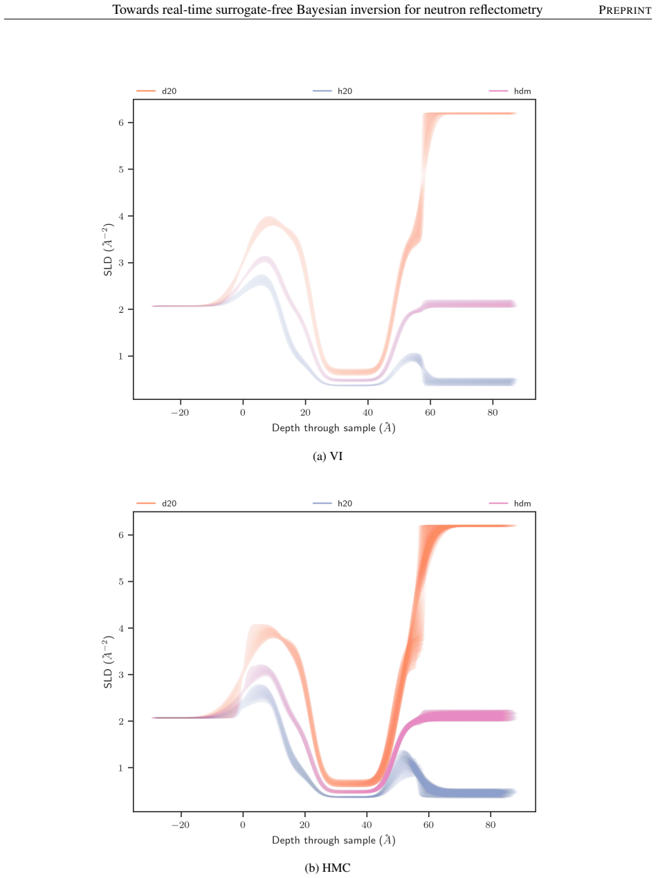
- Variational inference produces a full approximate posterior over 59 joint parameters, co-fitting four OLED devices with shared instrument parameters, in under 20 seconds per run, bringing UQ to the timescale of fast kinetic NR experiments.
- VI's mode-seeking tendency to understate posterior variance is acknowledged and demonstrated on a lipid bilayer benchmark against HMC, giving practitioners a concrete picture of the speed-versus-fidelity trade-off.
- The library makes the kernels, smearing options, gradients, just-in-time compilation, and GPU parallelism available so the demonstrated optimisation and inference schemes can be reproduced and extended.
Reading between the lines
- If the gradient route holds up, it plausibly transfers to any indirect scattering technique with a differentiable forward model — small-angle scattering, ellipsometry, grazing-incidence scattering — since nothing in the method is specific to reflectometry beyond the kernel; a direct test is re-running the same VI/HMC pipeline on those forward models.
- The seconds-scale runtime opens the door to closed-loop process control and active experimental design at the beamline without surrogates, for example using the VI posterior of one measurement to choose settings for the next; the paper gestures at this via Bayesian optimisation but does not demonstrate it.
- Because the surrogate q is chosen to be Gaussian, VI will understate uncertainty whenever the true posterior is multimodal or skewed, which the phase-loss degeneracy of reflectometry makes likely; a testable extension is a more flexible surrogate family such as mixtures or normalising flows to recover tails while keeping the runtime short.
- The posterior differences between OLED devices, such as the thicker oxide inferred for the 140°C-annealed sample, come from a single measurement each; replicate devices would reveal whether those differences are genuine sample variability or slack in the slab-model degrees of freedom.
Editorial analysis
A structured set of objections, weighed in public.
Referee Report
Summary. The paper presents refjax, an open-source JAX library that computes specular neutron reflectivity from an arbitrary slab model and, via automatic differentiation, exact gradients with respect to model parameters. These gradients are used to run gradient-based optimisation (Adam), Hamiltonian Monte Carlo (NUTS), and variational inference on NR inverse problems. The method is demonstrated on a crystalline quartz film on silicon (D17 instrument) and on a joint fit of four OLED devices (59 parameters), with an additional lipid bilayer benchmark in the Appendix. The authors report a posterior-mean χ² of 1.22 for quartz (better than the published 1.32), an OLED co-fit via VI in under 20 seconds on a 64-core workstation, and an ESS-per-iteration comparison indicating that NUTS converges where a sample-adaptive MCMC sampler appears to stall. The central claim is that exact gradients through the physical forward model provide a step-change in inference speed and sample efficiency compared with gradient-free MCMC, and that VI can deliver approximate UQ on the order of seconds.
Significance. If the central claim holds, the work is a significant practical contribution to NR analysis: it removes the need for surrogate models, provides a public code base (refjax), and opens the door to gradient-based Bayesian methods for a community that still largely uses Levenberg-Marquardt or gradient-free samplers. The paper is generally honest: it discloses the non-physical quartz oxide SLD, notes the mode-seeking variance underprediction of VI, and includes an external benchmark against refnx. The use of exact gradients through the Abeles model is conceptually clean and the released code makes the approach reproducible. However, the quantitative evidence for the headline speed/efficiency gains is currently incomplete. The ESS comparison is not cost-adjusted, and the VI timing has no same-hardware baseline, so the 'order of magnitude' and 'seconds rather than hours' claims are not yet established. The paper would be strengthened by a careful cost-adjusted benchmark on multiple datasets and posterior geometries.
major comments (4)
- [Section 3.1, Figure 6] The sample-efficiency comparison is reported as ESS per iteration, not ESS per wall-clock time. The text acknowledges that NUTS's per-sample cost is 'several times higher' than SA-MCMC, but no ratio is given. Because the Abstract claims 'order of magnitude gains in sample-efficiency' and the Introduction claims a 'step-change in inference speed', the comparison must be normalised by computational cost. Please report ESS per second (or per cost-normalised gradient evaluation) on the same hardware, and state the per-sample cost ratio. If the ratio is, say, 5–10×, the ESS-per-iteration advantage shown in Fig. 6 may disappear.
- [Section 3.2, OLED VI] The timing claim ('<20 seconds', 'seconds rather than hours') is based on a single run of VI on a 64-core Threadripper with no same-hardware comparison to HMC/NUTS or to a gradient-free sampler on the same 59-parameter problem. The 'hours' appears to come from typical literature experience rather than from measurement. Please provide a side-by-side wall-clock comparison (including total time for all 100 restarts) and report the elapsed time for each method on the same hardware and data. In addition, selecting the best of 100 restarts by maximum noisy ELBO can bias the chosen surrogate posterior; please report the spread of ELBO values across restarts and/or use a common random seed or a deterministic ELBO evaluation for the selection.
- [Section 1.2, Eq. (25), Table 1] The reported posterior widths and the VI-versus-HMC comparison are conditional on a Gaussian likelihood with variances taken from the count data and on the assumed slab model (layer count, Gaussian roughness, smearing kernel). The paper does not validate this likelihood against the data. For instance, the quartz posterior mean assigns a native-oxide SLD of 0.323 Å^-2, far from the physical value (~3.4), which the authors attribute to slab-model slack. This indicates sensitivity to the model class. Please add a posterior predictive check (e.g., simulating from the posterior and comparing to the observed data) and, ideally, a simulation-based calibration study to assess whether the reported posterior widths are trustworthy.
- [Section 3.1, Figure 6 and convergence diagnostics] The ESS plot is described as 'the effective sample size of a single parameter in a single chain' and no R-hat diagnostics are reported for the full parameter vector. The sample-efficiency claim should be supported by summary ESS and R-hat across all parameters and all chains, not just one trace. Please specify which parameter(s) are plotted, report the convergence diagnostics for the entire model, and ensure the plotted chain/parameter is representative rather than cherry-picked.
minor comments (7)
- [Introduction] 'complex multiplayer structures' should be 'multilayer structures'.
- [Section 3.1] 'numypro' is a typo for 'numpyro'.
- [Table 4] The background initial value '5.0' is inconsistent with its prior U(e^-20, 1×10^-7); presumably the intended value is 5.0×10^-7. Please correct.
- [Appendix B] 'D20' and 'H20' should be 'D2O' and 'H2O'.
- [Section 1.4] 'variation inference' should be 'variational inference'.
- [Figure 6 caption] The caption is ambiguous: it says 'each line is the effective sample size of a single parameter in a single chain'—please clarify which parameters/chains are shown and how many lines appear.
- [Abstract] The claim 'for the first time in NR, exact gradients through the reflectivity are computed' is stated as a fact. The authors may wish to soften this to 'to the best of our knowledge' and ensure the literature search covers adjacent fields (X-ray reflectometry, optical thin films) where AD has been used.
Circularity Check
No significant circularity: the forward model is the standard Abeles formalism, inference uses standard numpyro samplers, and benchmarks are external datasets; speed claims are benchmarking concerns, not circular reductions.
full rationale
The derivation chain is self-contained. The forward reflectivity model is the standard Abeles matrix formalism ('The Abeles matrix formalism [23] provides a physical model of the reflectivity'), not a parameter fitted to the data, and the claimed novelty is exact automatic-differentiation gradients through this fixed model. The inference algorithms (NUTS, Sample Adaptive MCMC, ADAM, VI) are standard implementations from numpyro and JAX, not bespoke constructions that encode the conclusions. The empirical comparisons use external datasets: D17 quartz data ('The reflectivity data were collected on the D17 neutron reflectivity instrument at the ILL'), ISIS OLED data, and a refnx lipid benchmark ('this system makes an ideal benchmark for comparison of new fitting methodologies'). Warm-starting HMC at the Adam optimum is explicitly disclosed ('The chain was initialised prior to the burn-in at the optimal value found by gradient descent'), and the reported χ²=1.22 is a same-data fit-quality measure, not an out-of-sample prediction; this is a benchmarking weakness but not circularity. The admitted limitations — higher per-sample NUTS cost and VI variance underprediction (Appendix C) — are transparent trade-offs, not hidden reductions of outputs to inputs. No load-bearing self-citation or imported uniqueness/ansatz is present; even the reference to [38] is only a data source and published baseline, not an argumentative premise.
Assumptions & free parameters
free parameters (5)
- VI surrogate initialization and schedule =
sigma_0=0.1, learning rate 0.05, 2000 iterations, 100 restarts
- HMC/NUTS chain budget =
1000 burn-in samples, 10 chains of 2000 samples
- Slab model layer counts and prior bounds =
quartz: 2 layers; OLED: 4 layers; uniform priors in Tables 1-4
- OLED shared smearing parameter =
posterior 5.56±0.06 percent
- LED per-device scale and shared background =
scale: 0.954, 1.02, 0.998, 0.963; background: 4.99e-07
assumptions (5)
- domain assumption The Abeles matrix formalism exactly describes specular reflectivity for the slab models used
- domain assumption The likelihood p(R|theta) is Gaussian with variances taken from measured count data
- domain assumption A Gaussian surrogate on an unconstrained space adequately represents the posterior for VI purposes
- standard math NUTS default adaptation (step size and mass matrix) is a correct and robust HMC implementation
- domain assumption The prior bounds in Tables 1-4 contain all physically plausible parameter values
Cite this review
Pith. "Pith review of Towards real-time surrogate-free Bayesian inversion for neutron reflectometry." pith.science (2026). https://pith.science/paper/V3JLAGRP
@misc{pith2026250906924,
  author       = {Pith},
  title        = {Pith review of: Towards real-time surrogate-free Bayesian inversion for neutron reflectometry},
  year         = {2026},
  howpublished = {\url{https://pith.science/paper/V3JLAGRP}},
  note         = {Machine review of arXiv:2509.06924}
}
read the original abstract
Neutron reflectometry (NR) is a key enabling technology for many areas of scientific development. Although the forward reflectivity model is well-known, inferring the physical properties of a sample from NR data requires the solution of an inverse problem. Increasingly, beamline scientists are using NR in fast kinetic configurations and probing highly-complex structures and interfaces, introducing significant uncertainty. Existing uncertainty quantification (UQ) approaches in NR, such as Markov-Chain Monte-Carlo (MCMC), suffer from poor sample efficiency and slow convergence times. Recently, surrogate machine learning models have been proposed as an alternative. However, physical intuition is lost when replacing governing equations with fast surrogates. Instead, we propose a rapid, surrogate-free Bayesian inversion for NR. Our approach offers a step-change in inference speed and efficiency. For the first time in NR, exact gradients through the reflectivity are computed, enabling highly performant gradient-based inference schemes: Hamiltonian Monte-Carlo offers significant advances in sample efficiency compared to MCMC. Variational inference enables approximate UQ on the order of seconds rather than hours. We demonstrate state-of-the-art performance on a thick oxide quartz film, and robust co-fitting performance in the high complexity regime of organic LED multilayer devices. Additionally, we provide an open-source library of reflectometry kernels in the python language.
Figures


Figures from the paper (11 more)



Reference graph
Works this paper leans on
-
[1]
M. W. Skoda. Recent developments in the application of x-ray and neutron reflectivity to soft-matter systems. Current Opinion in Colloid & Interface Science, 2019
work page 2019
-
[2]
B. J. Kirby, P. A. Kienzle, B. B. Maranville, N. F. Berk, J. Krycka, F. Heinrich, and C. Majkrzak. Phase-sensitive specular neutron reflectometry for imaging the nanometer scale composition depth profile of thin-film materials. Current Opinion in Colloid & Interface Science, 2012
work page 2012
-
[3]
A. Junghans, E. B. Watkins, R. D. Barker, S. Singh, M. J. Waltman, H. L. Smith, L. Pocivavsek, and J. Majewski. Analysis of biosurfaces by neutron reflectometry: From simple to complex interfaces.Biointerphases, 2015. 17 Towards real-time surrogate-free Bayesian inversion for neutron reflectometryPREPRINT
work page 2015
-
[4]
C. F. Majkrzak, J. W. Cable, J. Kwo, M. Hong, T. Shih, and J. V . Waszczak. Neutron diffraction studies of fe/cr superlattices.Journal of Applied Physics, 1988
work page 1988
- [5]
- [6]
-
[7]
L. A. Clifton, S. A. Holt, A. V . Hughes, E. L. Daulton, W. Arunmanee, F. Heinrich, S. Khalid, D. Jefferies, T. R. Charlton, J. R. Webster,et al. An accurate in vitro model of the e. coli envelope.Angewandte Chemie International Edition, 2015
work page 2015
-
[8]
J. Penfold and R. Thomas. The application of the specular reflection of neutrons to the study of surfaces and interfaces.Journal of Physics: Condensed Matter, 1990
work page 1990
Show all 43 references
-
[9]
A. R. Nelson and S. W. Prescott. refnx: neutron and x-ray reflectometry analysis in python.Applied Crystallogra- phy, 2019
2019
-
[10]
J. Woollam. Completeease, 2017
2017
-
[11]
Levenberg
K. Levenberg. A method for the solution of certain non-linear problems in least squares.Quarterly of Applied Mathematics, 1944
1944
-
[12]
D. W. Marquardt. An algorithm for least-squares estimation of nonlinear parameters.Journal of the Society for Industrial and Applied Mathematics, 1963
1963
-
[13]
Nocedal and S
J. Nocedal and S. J. Wright.Numerical Optimization. Springer Series in Operations Research and Financial Engineering. Springer, 2nd edition, 2006
2006
-
[14]
Storn and K
R. Storn and K. Price. Differential evolution - a simple and efficient heuristic for global optimization over continuous spaces.Journal of Global Optimization, 1997
1997
-
[15]
Eberhart and J
R. Eberhart and J. Kennedy. A new optimizer using particle swarm theory. InMHS’95. Proceedings of the sixth international symposium on micro machine and human science. IEEE, 1995
1995
-
[16]
Metropolis, A
N. Metropolis, A. W. Rosenbluth, M. N. Rosenbluth, A. H. Teller, and E. Teller. Equation of state calculations by fast computing machines.The Journal of Chemical Physics, 1953
1953
-
[17]
W. K. Hastings. Monte carlo sampling methods using Markov chains and their applications.Biometrika, 1970
1970
-
[18]
Skilling
J. Skilling. Nested sampling.Bayesian inference and maximum entropy methods in science and engineering, 2004
2004
-
[19]
Doucet, R
M. Doucet, R. K. Archibald, and W. T. Heller. Machine learning for neutron reflectometry data analysis of two-layer thin films.Machine Learning: Science and Technology, 2021
2021
-
[20]
Hinderhofer, A
A. Hinderhofer, A. Greco, V . Starostin, V . Munteanu, L. Pithan, A. Gerlach, and F. Schreiber. Machine learning for scattering data: strategies, perspectives and applications to surface scattering.Applied Crystallography, 2023
2023
-
[21]
Pithan, V
L. Pithan, V . Starostin, D. Mare ˇcek, L. Petersdorf, C. Völter, V . Munteanu, M. Jankowski, O. Konovalov, A. Gerlach, A. Hinderhofer,et al. Closing the loop: autonomous experiments enabled by machine-learning-based online data analysis in synchrotron beamline environments.Sy...
2023
-
[22]
Starostin, M
V . Starostin, M. Dax, A. Gerlach, A. Hinderhofer, Á. Tejero-Cantero, and F. Schreiber. Fast and reliable probabilistic reflectometry inversion with prior-amortized neural posterior estimation.Science Advances, 2025
2025
-
[23]
Abelès.La théorie générale des couches minces
F. Abelès.La théorie générale des couches minces. PhD thesis, Université de Paris, 1949
1949
-
[24]
D. P. Kingma. Adam: A method for stochastic optimization.arXiv preprint arXiv:1412.6980, 2014
2014 arXiv
-
[25]
G. Hinton. Lecture 6e rmsprop: Divide the gradient by a running average of its recent magnitude. https: //www.cs.toronto.edu/~tijmen/csc321/slides/lecture_slides_lec6.pdf, 2012. Coursera: Neural Networks for Machine Learning. 18 Towards real-time surrogate-free Bayesian invers...
2012
-
[26]
Betancourt
M. Betancourt. A conceptual introduction to Hamiltonian Monte Carlo.arXiv preprint arXiv:1701.02434, 2017
2017 arXiv
-
[27]
D. M. Blei, A. Kucukelbir, and J. D. McAuliffe. Variational inference: A review for statisticians.Journal of the American statistical Association, 2017
2017
-
[28]
Hairer, M
E. Hairer, M. Hochbruck, A. Iserles, and C. Lubich. Geometric numerical integration.Oberwolfach Reports, 2006
2006
-
[29]
M. D. Hoffman, A. Gelman,et al. The no-u-turn sampler: adaptively setting path lengths in Hamiltonian Monte Carlo.J. Mach. Learn. Res., 2014
2014
-
[30]
M. I. Jordan, Z. Ghahramani, T. S. Jaakkola, and L. K. Saul. An introduction to variational methods for graphical models.Machine Learning, 1999
1999
-
[31]
M. D. Hoffman, D. M. Blei, C. Wang, and J. Paisley. Stochastic variational inference.the Journal of machine Learning research, 2013
2013
-
[32]
Yin and M
M. Yin and M. Zhou. Semi-implicit variational inference. InInternational conference on machine learning. PMLR, 2018
2018
-
[33]
D. P. Kingma and M. Welling. Auto-encoding variational bayes. InInternational Conference on Learning Representations (ICLR), 2014
2014
-
[34]
Bradbury, R
J. Bradbury, R. Frostig, P. Hawkins, M. J. Johnson, C. Leary, D. Maclaurin, G. Necula, A. Paszke, J. VanderPlas, S. Wanderman-Milne, and Q. Zhang. JAX: composable transformations of Python+NumPy programs, 2018
2018
-
[35]
Rader, T
J. Rader, T. Lyons, and P. Kidger. Optimistix: modular optimisation in jax and equinox.arXiv preprint arXiv:2402.09983, 2024
2024 arXiv
-
[36]
Babuschkin, K
DeepMind, I. Babuschkin, K. Baumli, A. Bell, S. Bhupatiraju, J. Bruce, P. Buchlovsky, D. Budden, T. Cai, A. Clark, I. Danihelka, A. Dedieu, C. Fantacci, J. Godwin, C. Jones, R. Hemsley, T. Hennigan, M. Hessel, S. Hou, S. Kapturowski, T. Keck, I. Kemaev, M. King, M. Kunesch, L....
2020
-
[37]
D. Phan, N. Pradhan, and M. Jankowiak. Composable effects for flexible and accelerated probabilistic program- ming in numpyro.arXiv preprint arXiv:1912.11554, 2019
1912 arXiv
-
[38]
Gutfreund, T
P. Gutfreund, T. Saerbeck, M. A. Gonzalez, E. Pellegrini, M. Laver, C. Dewhurst, and R. Cubitt. Towards general- ized data reduction on a chopper-based time-of-flight neutron reflectometer.Journal of Applied Crystallography, 2018
2018
-
[39]
A. Hajian. Efficient cosmological parameter estimation with hamiltonian monte carlo technique.Physical Review D—Particles, Fields, Gravitation, and Cosmology, 2007
2007
-
[40]
M. Tinto. Gravitational wave searches with pulsar timing arrays: Cancellation of clock and ephemeris noises. Physical Review D, 2018
2018
-
[41]
M. Zhu. Sample Adaptive MCMC.Advances in Neural Information Processing Systems, 2019
2019
-
[42]
Lanfear, X
R. Lanfear, X. Hua, and D. L. Warren. Estimating the effective sample size of tree topologies from Bayesian phylogenetic analyses.Genome biology and evolution, 2016
2016
-
[43]
B. Ru, M. A. Osborne, M. McLeod, and D. Granziol. Fast information-theoretic Bayesian optimisation. In International Conference on Machine Learning. PMLR, 2018. 19 Towards real-time surrogate-free Bayesian inversion for neutron reflectometryPREPRINT A Posterior distributions P...
2018
Reviewed August 4, 2026 · model on record in the stance chip above.
Discussion (0). Continue with ORCID to comment.