REVIEW 4 major objections 4 minor 172 references
Interpretable Embeddings with Sparse Autoencoders: A Data Analysis Toolkit
T0 review · 4 major / 4 minor · reviewed 2026-08-03 · deepseek-v4-flash
Pith's one-line read Sparse autoencoder embeddings, whose dimensions are named concepts, make text-corpus analysis cheaper, more reliable, and more controllable than LLM labeling or dense embeddings.
desk verdict A well-executed empirical toolkit paper demonstrating SAE embeddings' value across four data-analysis tasks, with a genuinely testable Tulu-3 case study; the main weakness is unquantified latent-label quality, an addressable limitation rather than a fatal flaw. read the letter →
The pith
A machine-rendered reading of the paper's core claim, the machinery that carries it, and where it could break.
The reading
What carries the argument
SAE embeddings: a document is embedded as the max over token-level sparse autoencoder activations from a reader LLM, so each of roughly 65,000 dimensions is a fixed, human-readable concept (a 'latent' with an auto-generated label, produced by prompting an LLM with ten activating and ten non-activating phrases). These dimensions supply a large, fixed hypothesis space of concept detectors. Frequencies of binarized dimensions enable dataset diffing; pairwise normalized pointwise mutual information between dimensions, filtered by low label similarity, surfaces surprising correlations; restricting the embedding to query-relevant dimensions gives controllable clustering and retrieval.
What would settle it
Take a held-out corpus with known concept labels (e.g., the synthetic tone and genre datasets plus an out-of-distribution set) and measure precision/recall of each binarized SAE dimension against the label; if a substantial fraction of high-frequency dimensions have near-chance precision, the label layer fails. Alternatively, rerun all four tasks with a second independently labeled SAE on the same reader model and check whether the top dataset differences, correlations, clusters, and retrieval rankings replicate; non-replication would show the results are tied to one label set rather than to t
Extended reading notes
Core claim
At the center is a simple construction: feed each document to a reader LLM, extract per-token internal activations, apply a pretrained sparse autoencoder whose 65,536 dimensions have been labeled with concept descriptions, and max-pool activations across tokens. The resulting vector is an embedding whose axes are named properties (e.g., 'asks a clarifying question,' 'personifies objects'), and binarizing it turns the SAE into a mass labeler for thousands of concepts. The paper claims this construction outperforms LLM-based baselines on dataset diffing and correlation discovery—finding larger, judge-verified differences at 2–8x lower token cost and recovering injected correlations that an LLM
Load-bearing premise
The reused auto-generated labels for the 61,521 SAE dimensions are accurate, monosemantic, and stable on out-of-distribution corpora; if many labels fire on the wrong concepts or absorb multiple meanings, the reliability and controllability claims weaken—the paper's own Limitations section flags feature absorption without quantifying its effect.
Editorial extensions
If this is right
- A single pretrained SAE plus reader LLM can replace repeated LLM prompting for dataset comparison: once the embedding is built, datasets can be diffed and re-diffed at near-zero marginal cost.
- Differences and correlations found this way come with human-readable names, so a practitioner can go from a statistical signal to a testable hypothesis without a separate interpretation step.
- Filtering the embedding to concept-relevant dimensions changes what clustering and retrieval optimize for: instead of topic similarity, a user can cluster by reasoning style, tone, or formatting.
- The same tool can audit training data: identifying prompt features correlated with unwanted response phrases, then generating new prompts to confirm the model has learned the correlation.
- Because the embeddings are reused across comparisons, adding more models or datasets to an analysis is cheaper than rerunning LLM baselines.
- Cost-effectiveness is most pronounced in multi-model settings, where the SAE embedding is computed once and then compared across many targets.
Reading between the lines
- If the label layer is trustworthy, the reader-model SAE becomes a shared measurement instrument: one could audit any model's outputs without access to that model's internals, which would make cross-company behavioral comparisons much cheaper.
- The controllability result suggests a natural extension: composing multiple property queries into a single retrieval or clustering objective could support open-ended 'find me texts that are X but not Y' analyses, which dense embeddings cannot express.
- Since performance drops on corpora far from the SAE's training distribution, a testable extension is to train or select domain-specific reader SAEs and pool their latents; the paper hints at this but does not evaluate it.
- The reliability of every downstream number inherits from label accuracy, so an automated calibration pass—relabeling or pruning low-precision latents per corpus—would likely sharpen the paper's results; the authors acknowledge feature absorption but do not quantify its effect.
Editorial analysis
A structured set of objections, weighed in public.
Referee Report
Summary. The paper proposes using pretrained sparse autoencoders (SAEs) on an LLM's hidden states to construct 'SAE embeddings': per-document vectors whose dimensions are labeled, human-interpretable concepts. It applies these embeddings to four data-analysis tasks — dataset diffing, correlation mining, clustering, and property-based retrieval — and reports that SAE embeddings are more cost-effective and reliable than LLM-based annotation and more controllable than dense embeddings. Two case studies apply the method to OpenAI model generations and to finding a spurious 'I hope it is correct' trigger in Tulu-3's post-training data. The core method is clearly specified, code is released, and each task includes at least one validation component; the Tulu-3 case study generates new prompts to verify the discovered trigger.
Significance. If the central claims hold, this paper would make a useful contribution: it shows that a single reader model's SAE can serve as a reusable, interpretable labeler across many text-analysis tasks, and it provides a concrete toolkit with code. Strengths include the explicit task-specific validations, the synthetic injection experiments for correlations, the cost comparison with token counts, and the Tulu-3 trigger study, which is genuinely testable and tested with newly generated prompts. The paper is also honest in its Limitations section about feature absorption and sensitivity to the SAE's training distribution. However, the strength of the headline claim — 'more reliable than LLMs' — depends on the quality of the 61,521 reused latent descriptions, and that dependency is not quantified for the specific latents used in the headline experiments. The evidence for label quality in Appendix I is partial, samples an unrepresentative subset of latents, and uses an LLM judge as ground truth. These issues are fixable but currently leave a gap between the evidence and the abstract's reliability claim.
major comments (4)
- [§3, Limitations, and Appendix I] The central reliability claim depends on the 61,521 reused Goodfire latent descriptions. The paper acknowledges in Limitations that SAEs are 'imperfect labelers due to feature absorption' but does not quantify absorption or label error for the latents that actually drive the reported results. Appendix I evaluates latent-as-classifier F1 on Pile/arXiv/GPT-5, but it samples only 100 latents active in >10% of documents, which is not the same distribution as the top-frequency-difference latents (§4.1), high-NPMI pairs (§4.2), or retrieval latents (§4.4). Additionally, the F1 ground truth is an LLM judge, which is partly circular with the LLM-based label-generation process. I would like to see a targeted evaluation: sample latents from the top of each task-specific ranking, measure precision/recall against human annotations, and report how many hypotheses would be invalidated by absorption or
- [§4.1 and Appendix D.3] The abstract's 'more reliable than LLMs' is not uniformly supported by the paper's own ground-truth diffing comparison. In Appendix D.3, the SAE achieves average surface similarity 0.75 (movies) and 0.80 (tones), while the GPT-5 baseline achieves 0.90 (movies) and 0.78 (tones). Thus on one of the two grounded settings the LLM baseline is stronger. The later verification-rate results (Figure 11) support a more specific claim: SAE-generated hypotheses have higher judge-verified frequency differences in multi-model settings. The paper should qualify the 'more reliable' claim to this setting, or provide additional evidence that the SAE is more reliable across the four tasks as a whole.
- [§4.2, Figure 4] The 'verified NPMI' evaluation in Figure 4 is partly self-referential. Latent labels are produced by an LLM, and the judge that verifies their presence is also an LLM. The CDF therefore measures consistency between the latent label and the LLM judge, not necessarily ground-truth semantic correlation. The synthetic injection experiments provide a genuinely external anchor and are a strength, but the real-world correlation signal (CivilComments, Pile) would be more convincing with a human-annotated subset or an independent, non-LLM validation. Without this, the claim that SAEs 'identify biases more reliably' is only as strong as the unverified label quality.
- [§4.4, Tables 23–28] The retrieval results show substantial query-level variance that is not discussed in the main text. For example, on ChatbotArena prompts the query about fictional story generation drops from 0.719 (OpenAI+LLM) to 0.110 (SAE), while 'user includes emojis' improves from 0.066 to 0.480. These swings suggest that the SAE's advantage is concentrated in certain property types (formatting, repetition, multilingual patterns) and not in others (narrative, philosophical content). Reporting aggregate MAP alone may overstate the 'generally outperform or match' conclusion. I would like an error analysis or at least a sentence acknowledging that the SAE is better for some property families and worse for others.
minor comments (4)
- [§3] 'we find 61521 existing latent descriptions that we reuse' is ungrammatical; suggest 'we reuse 61,521 existing latent descriptions'.
- [§4.1, Table 3] The cost table reports token usage including latent relabeling, but the SAE's fixed cost of obtaining the pretrained SAE and labels is excluded. This is acceptable if the SAE is reused across many tasks, but the paper should state this amortization assumption explicitly in the main text, not only in the caption.
- [§4.3, Figure 5] The cluster labels in Figure 5 are useful, but the scores in the 'Acc.' column are not defined until later in the text. Please define 'Acc.' and the z-score metric when the figure is first referenced, so that a reader does not have to jump to §4.3 or Appendix F.
- [Appendix F.4] The appendix reports that SAEs 'were unable to find a good combination of queries and k' for sentiment and emotion clustering. This is an honest negative result, but it is not mentioned in the main-text limitations. A one-sentence acknowledgment in §4.3 would help readers calibrate the controllability claim.
Circularity Check
No load-bearing circularity: SAE embeddings are applied to fixed reused latents and checked against external anchors; main threats are unquantified label error and LLM-judge self-referentiality, not construction-level circularity.
full rationale
The paper's derivation chain does not reduce to its inputs. SAE embeddings are produced by max-pooling activations of a fixed, reused Goodfire SAE (Section 3: 'we find 61521 existing latent descriptions that we reuse'), and the headline findings are compared against external anchors: movie genre labels, synthetic tone shifts, injected correlations, GSM8k solutions, and newly generated Tulu-3 prompts. The Tulu 'I hope it is correct' trigger was not read off the SAE; it was verified by generating new prompts varying the hypothesized axes (Figures 8-9), so it is an independent test. Retrieval uses LLM-judged query relevance, but the SAE scores do not fit those judgments; selection of hyperparameters (temperature, number of phrases) on the evaluated datasets is a test-set tuning concern, not a circular reduction. The only overlapping-author citation, [53] (Kantamneni et al., with coauthor Nanda), appears as a related-work example and is not load-bearing. The real limitation—unquantified feature absorption and label inaccuracy on the reused latents, acknowledged in Limitations ('imperfect labelers due to feature absorption')—undermines external validity and makes the LLM-judged F1 evaluation in Appendix I partly self-referential, but it does not make any reported result equal to a fitted input by construction. Hence no circular step meets the quoted-reduction bar; score 2 for a minor non-load-bearing self-citation and self-referential evaluation concerns.
Assumptions & free parameters
free parameters (5)
- diffing frequency-difference threshold =
0.03
- correlation cutoffs (NPMI, label similarity) =
NPMI > 0.6/0.7, sim < 0.2
- retrieval temperature T =
selected by best MAP averaged over datasets; range 0.01-1.5
- number of LLM query-expansion phrases =
selected by best MAP averaged over datasets; range 1-20
- top-k latents for targeted clustering =
k=100
assumptions (5)
- domain assumption Each SAE latent’s label accurately describes the concept that activates it, and activation indicates presence of that concept in text.
- domain assumption LLM-generated latent labels (EleutherAI-style autointerp and Goodfire’s precomputed descriptions) are valid across the corpora analyzed.
- domain assumption LLM judges correctly detect whether a text has a hypothesized property.
- domain assumption Max-pooling SAE activations over tokens preserves the document-level properties needed for diffing, correlation, clustering, and retrieval.
- domain assumption A reader SAE trained on Llama 3.3 70B layer 50 hidden states from LMSYS-Chat-1M transfers to arbitrary text domains (Pile, arXiv, Reddit, etc.).
Cite this review
Pith. "Pith review of Interpretable Embeddings with Sparse Autoencoders: A Data Analysis Toolkit." pith.science (2026). https://pith.science/paper/VSTYNZ3G
@misc{pith2026251210092,
  author       = {Pith},
  title        = {Pith review of: Interpretable Embeddings with Sparse Autoencoders: A Data Analysis Toolkit},
  year         = {2026},
  howpublished = {\url{https://pith.science/paper/VSTYNZ3G}},
  note         = {Machine review of arXiv:2512.10092}
}
read the original abstract
Analyzing large-scale text corpora is a core challenge in machine learning, crucial for tasks like identifying undesirable model behaviors or biases in training data. Current methods often rely on costly LLM-based techniques (e.g. annotating dataset differences) or dense embedding models (e.g. for clustering), which lack control over the properties of interest. We propose using sparse autoencoders (SAEs) to create SAE embeddings: representations whose dimensions map to interpretable concepts. Through four data analysis tasks, we show that SAE embeddings are more cost-effective and reliable than LLMs and more controllable than dense embeddings. Using the large hypothesis space of SAEs, we can uncover insights such as (1) semantic differences between datasets and (2) unexpected concept correlations in documents. For instance, by comparing model responses, we find that Grok-4 clarifies ambiguities more often than nine other frontier models. Relative to LLMs, SAE embeddings uncover bigger differences at 2-8x lower cost and identify biases more reliably. Additionally, SAE embeddings are controllable: by filtering concepts, we can (3) cluster documents along axes of interest and (4) outperform dense embeddings on property-based retrieval. Using SAE embeddings, we study model behavior with two case studies: investigating how OpenAI model behavior has changed over time and finding "trigger" phrases learned by Tulu-3 (Lambert et al., 2024) from its training data. These results position SAEs as a versatile tool for unstructured data analysis and highlight the neglected importance of interpreting models through their data.
Figures


Figures from the paper (26 more)




Reference graph
Works this paper leans on
-
[1]
Miranda, Alisa Liu, Nouha Dziri, Shane Lyu, Yuling Gu, Saumya Malik, Victoria Graf, Jena D
Nathan Lambert, Jacob Morrison, Valentina Pyatkin, Shengyi Huang, Hamish Ivison, Faeze Brahman, Lester James V . Miranda, Alisa Liu, Nouha Dziri, Shane Lyu, Yuling Gu, Saumya Malik, Victoria Graf, Jena D. Hwang, Jiangjiang Yang, Ronan Le Bras, Oyvind Tafjord, Chris Wilhelm, Luca Soldaini, Noah A. Smith, Yizhong Wang, Pradeep Dasigi, and Hannaneh Hajishirz...
2024
-
[2]
Introducing docent
Kevin Meng, Vincent Huang, Jacob Steinhardt, and Sarah Schwettmann. Introducing docent. https://transluce.org/introducing-docent, March 2025
2025
-
[3]
Semantic operators: A declarative model for rich, ai-based data processing, 2025
Liana Patel, Siddharth Jha, Melissa Pan, Harshit Gupta, Parth Asawa, Carlos Guestrin, and Matei Zaharia. Semantic operators: A declarative model for rich, ai-based data processing, 2025
2025
-
[4]
Parameswaran, and Eugene Wu
Shreya Shankar, Tristan Chambers, Tarak Shah, Aditya G. Parameswaran, and Eugene Wu. Docetl: Agentic query rewriting and evaluation for complex document processing, 2025
2025
-
[5]
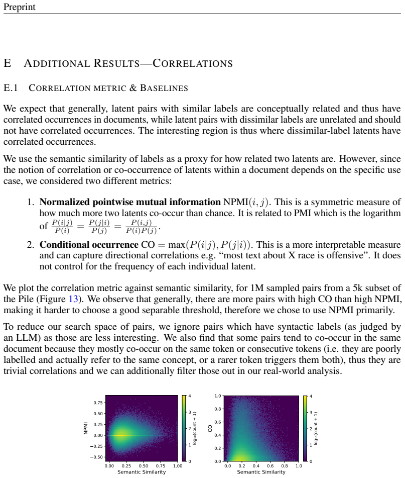
Negar Arabzadeh and Charles L.A. Clarke. A human-ai comparative analysis of prompt sensitivity in llm-based relevance judgment. InProceedings of the 48th International ACM SIGIR Conference on Research and Development in Information Retrieval, SIGIR ’25, page 2784–2788. ACM, July 2025
2025
-
[6]
The order effect: Investigating prompt sensitivity to input order in llms, 2025
Bryan Guan, Tanya Roosta, Peyman Passban, and Mehdi Rezagholizadeh. The order effect: Investigating prompt sensitivity to input order in llms, 2025
2025
-
[7]
Sentence-bert: Sentence embeddings using siamese bert- networks, 2019
Nils Reimers and Iryna Gurevych. Sentence-bert: Sentence embeddings using siamese bert- networks, 2019
2019
-
[8]
Sparse autoencoders find highly interpretable features in language models, 2023
Hoagy Cunningham, Aidan Ewart, Logan Riggs, Robert Huben, and Lee Sharkey. Sparse autoencoders find highly interpretable features in language models, 2023
2023
Show all 172 references
-
[9]
Towards monosemanticity: Decomposing language models with dictionary learning.Transformer Circuits Thread, 2023
Trenton Bricken, Adly Templeton, Joshua Batson, Brian Chen, Adam Jermyn, Tom Con- erly, Nick Turner, Cem Anil, Carson Denison, Amanda Askell, Robert Lasenby, Yifan Wu, Shauna Kravec, Nicholas Schiefer, Tim Maxwell, Nicholas Joseph, Zac Hatfield-Dodds, Alex Tamkin, Karina Nguye...
2023
-
[10]
Daniel Freeman, Theodore R
Adly Templeton, Tom Conerly, Jonathan Marcus, Jack Lindsey, Trenton Bricken, Brian Chen, Adam Pearce, Craig Citro, Emmanuel Ameisen, Andy Jones, Hoagy Cunningham, Nicholas L Turner, Callum McDougall, Monte MacDiarmid, C. Daniel Freeman, Theodore R. Sumers, Edward Rees, Joshua ...
2024
-
[11]
A vector space model for automatic indexing
Gerard Salton, Anita Wong, and Chung-Shu Yang. A vector space model for automatic indexing. Commun. ACM, 18:613–620, 1975
1975
-
[12]
Term weighting approaches in automatic text retrieval
Gerard Salton and Chris Buckley. Term weighting approaches in automatic text retrieval. Technical report, USA, 1987
1987
-
[13]
Semaxis: A lightweight framework to charac- terize domain-specific word semantics beyond sentiment, 2018
Jisun An, Haewoon Kwak, and Yong-Yeol Ahn. Semaxis: A lightweight framework to charac- terize domain-specific word semantics beyond sentiment, 2018
2018
-
[14]
The polar framework: Polar opposites enable interpretability of pre-trained word embeddings, 2020
Binny Mathew, Sandipan Sikdar, Florian Lemmerich, and Markus Strohmaier. The polar framework: Polar opposites enable interpretability of pre-trained word embeddings, 2020
2020
-
[15]
Frameaxis: characterizing mi- croframe bias and intensity with word embedding.PeerJ Computer Science, 7:e644, July 2021
Haewoon Kwak, Jisun An, Elise Jing, and Yong-Yeol Ahn. Frameaxis: characterizing mi- croframe bias and intensity with word embedding.PeerJ Computer Science, 7:e644, July 2021
2021
-
[16]
Learning interpretable word embeddings via bidirectional alignment of dimensions with semantic concepts.Information Processing & Management, 59(3):102925, 2022
Lütfi Kerem ¸ Senel, Furkan ¸ Sahinuç, Veysel Yücesoy, Hinrich Schütze, Tolga Çukur, and Aykut Koç. Learning interpretable word embeddings via bidirectional alignment of dimensions with semantic concepts.Information Processing & Management, 59(3):102925, 2022
2022
-
[17]
Sensepolar: Word sense aware interpretability for pre-trained contextual word embeddings, 2023
Jan Engler, Sandipan Sikdar, Marlene Lutz, and Markus Strohmaier. Sensepolar: Word sense aware interpretability for pre-trained contextual word embeddings, 2023
2023
-
[18]
Morris, Richard Antonello, Ion Stoica, Alexander G
Vinamra Benara, Chandan Singh, John X. Morris, Richard Antonello, Ion Stoica, Alexander G. Huth, and Jianfeng Gao. Crafting interpretable embeddings by asking llms questions, 2024
2024
-
[19]
Charles O’Neill, Christine Ye, Kartheik Iyer, and John F. Wu. Disentangling dense embeddings with sparse autoencoders, 2024
2024
-
[20]
Interpret and control dense retrieval with sparse latent features, 2025
Hao Kang, Tevin Wang, and Chenyan Xiong. Interpret and control dense retrieval with sparse latent features, 2025
2025
-
[21]
Sparse autoencoders for hypothesis generation, 2025
Rajiv Movva, Kenny Peng, Nikhil Garg, Jon Kleinberg, and Emma Pierson. Sparse autoencoders for hypothesis generation, 2025
2025
-
[22]
Vibecheck: Discover and quantify qualitative differences in large language models, 2025
Lisa Dunlap, Krishna Mandal, Trevor Darrell, Jacob Steinhardt, and Joseph E Gonzalez. Vibecheck: Discover and quantify qualitative differences in large language models, 2025
2025
-
[23]
Blair Yang, Fuyang Cui, Keiran Paster, Jimmy Ba, Pashootan Vaezipoor, Silviu Pitis, and Michael R. Zhang. Report cards: Qualitative evaluation of language models using natural language summaries, 2024
2024
-
[24]
Zico Kolter, and Zhuang Liu
Mingjie Sun, Yida Yin, Zhiqiu Xu, J. Zico Kolter, and Zhuang Liu. Idiosyncrasies in large language models, 2025
2025
-
[25]
Llm comparator: Visual analytics for side-by-side evaluation of large language models, 2024
Minsuk Kahng, Ian Tenney, Mahima Pushkarna, Michael Xieyang Liu, James Wexler, Emily Reif, Krystal Kallarackal, Minsuk Chang, Michael Terry, and Lucas Dixon. Llm comparator: Visual analytics for side-by-side evaluation of large language models, 2024
2024
-
[26]
Automatically interpreting millions of features in large language models, 2024
Gonçalo Paulo, Alex Mallen, Caden Juang, and Nora Belrose. Automatically interpreting millions of features in large language models, 2024
2024
-
[27]
Llama 3.3 model card
Meta AI. Llama 3.3 model card. https://github.com/meta-llama/ llama-models/blob/main/models/llama3_3/MODEL_CARD.md, 2024. Ac- cessed: 2025-08-04
2024
-
[28]
P Xing, Joseph E
Lianmin Zheng, Wei-Lin Chiang, Ying Sheng, Tianle Li, Siyuan Zhuang, Zhanghao Wu, Yonghao Zhuang, Zhuohan Li, Zi Lin, Eric. P Xing, Joseph E. Gonzalez, Ion Stoica, and Hao Zhang. Lmsys-chat-1m: A large-scale real-world llm conversation dataset, 2023
2023
-
[29]
Understanding and steering llama 3 with sparse autoencoders, 2024
Thomas McGrath, Daniel Balsam, Myra Deng, and Eric Ho. Understanding and steering llama 3 with sparse autoencoders, 2024
2024
-
[30]
Gemini 2.5: Pushing the frontier with advanced reasoning, multimodality, long context, and next generation agentic capabilities, 2025
Google Gemini Team. Gemini 2.5: Pushing the frontier with advanced reasoning, multimodality, long context, and next generation agentic capabilities, 2025. 12 Preprint
2025
-
[31]
Openai embeddings
OpenAI. Openai embeddings. https://platform.openai.com/docs/guides/ embeddings, 2024. Accessed: July 2025
2024
-
[32]
Gonzalez, and Serena Yeung-Levy
Lisa Dunlap, Yuhui Zhang, Xiaohan Wang, Ruiqi Zhong, Trevor Darrell, Jacob Steinhardt, Joseph E. Gonzalez, and Serena Yeung-Levy. Describing differences in image sets with natural language. InConference on Computer Vision and Pattern Recognition (CVPR), 2024
2024
-
[33]
Maas, Raymond E
Andrew L. Maas, Raymond E. Daly, Peter T. Pham, Dan Huang, Andrew Y . Ng, and Christopher Potts. Learning word vectors for sentiment analysis. InProceedings of the 49th Annual Meeting of the Association for Computational Linguistics: Human Language Technologies, pages 142–150,...
2011
-
[34]
P Xing, Hao Zhang, Joseph E
Lianmin Zheng, Wei-Lin Chiang, Ying Sheng, Siyuan Zhuang, Zhanghao Wu, Yonghao Zhuang, Zi Lin, Zhuohan Li, Dacheng Li, Eric. P Xing, Hao Zhang, Joseph E. Gonzalez, and Ion Stoica. Judging llm-as-a-judge with mt-bench and chatbot arena, 2023
2023
-
[35]
Llava-next: Improved reasoning, ocr, and world knowledge, January 2024
Haotian Liu, Chunyuan Li, Yuheng Li, Bo Li, Yuanhan Zhang, Sheng Shen, and Yong Jae Lee. Llava-next: Improved reasoning, ocr, and world knowledge, January 2024
2024
-
[36]
Measuring coding challenge competence with apps.NeurIPS, 2021
Dan Hendrycks, Steven Basart, Saurav Kadavath, Mantas Mazeika, Akul Arora, Ethan Guo, Collin Burns, Samir Puranik, Horace He, Dawn Song, and Jacob Steinhardt. Measuring coding challenge competence with apps.NeurIPS, 2021
2021
-
[37]
Gerlof J. Bouma. Normalized (pointwise) mutual information in collocation extraction. 2009
2009
-
[38]
Nu- anced metrics for measuring unintended bias with real data for text classification.CoRR, abs/1903.04561, 2019
Daniel Borkan, Lucas Dixon, Jeffrey Sorensen, Nithum Thain, and Lucy Vasserman. Nu- anced metrics for measuring unintended bias with real data for text classification.CoRR, abs/1903.04561, 2019
1903 arXiv
-
[39]
Smith, Luke Zettlemoyer, and Tao Yu
Hongjin Su, Weijia Shi, Jungo Kasai, Yizhong Wang, Yushi Hu, Mari Ostendorf, Wen tau Yih, Noah A. Smith, Luke Zettlemoyer, and Tao Yu. One embedder, any task: Instruction-finetuned text embeddings, 2023
2023
-
[40]
Training verifiers to solve math word problems.arXiv preprint arXiv:2110.14168, 2021
Karl Cobbe, Vineet Kosaraju, Mohammad Bavarian, Mark Chen, Heewoo Jun, Lukasz Kaiser, Matthias Plappert, Jerry Tworek, Jacob Hilton, Reiichiro Nakano, Christopher Hesse, and John Schulman. Training verifiers to solve math word problems.arXiv preprint arXiv:2110.14168, 2021
2021 arXiv
-
[41]
Ms marco: A human generated machine reading comprehension dataset
Payal Bajaj, Daniel Campos, Nick Craswell, Li Deng, Jianfeng Gao, Xiaodong Liu, Rangan Majumder, Andrew McNamara, Bhaskar Mitra, Tri Nguyen, Mir Rosenberg, Xia Song, Alina Stoica, Saurabh Tiwary, and Tong Wang. Ms marco: A human generated machine reading comprehension dataset....
2016
-
[42]
Mteb: Massive text embedding benchmark.arXiv preprint arXiv:2210.07316, 2022
Niklas Muennighoff, Nouamane Tazi, Loïc Magne, and Nils Reimers. Mteb: Massive text embedding benchmark.arXiv preprint arXiv:2210.07316, 2022
2022 arXiv
-
[43]
Mmteb: Massive multilingual text embedding benchmark
Kenneth Enevoldsen, Isaac Chung, Imene Kerboua, Márton Kardos, Ashwin Mathur, David Stap, Jay Gala, Wissam Siblini, Dominik Krzemi ´nski, Genta Indra Winata, Saba Sturua, Saiteja Utpala, Mathieu Ciancone, Marion Schaeffer, Gabriel Sequeira, Diganta Misra, Shreeya Dhakal, Jonat...
2025
-
[44]
Description-based text similarity, 2024
Shauli Ravfogel, Valentina Pyatkin, Amir DN Cohen, Avshalom Manevich, and Yoav Goldberg. Description-based text similarity, 2024
2024
-
[45]
Llama-nemotron: Efficient reasoning models, 2025
Akhiad Bercovich, Itay Levy, Izik Golan, Mohammad Dabbah, Ran El-Yaniv, Omri Puny, Ido Galil, Zach Moshe, Tomer Ronen, Najeeb Nabwani, Ido Shahaf, Oren Tropp, Ehud Karpas, Ran Zilberstein, Jiaqi Zeng, Soumye Singhal, Alexander Bukharin, Yian Zhang, Tugrul Konuk, Ger- ald Shen,...
2025
-
[46]
The pile: An 800gb dataset of diverse text for language modeling, 2020
Leo Gao, Stella Biderman, Sid Black, Laurence Golding, Travis Hoppe, Charles Foster, Jason Phang, Horace He, Anish Thite, Noa Nabeshima, Shawn Presser, and Connor Leahy. The pile: An 800gb dataset of diverse text for language modeling, 2020
2020
-
[47]
Clement, Matthew Bierbaum, Kevin P
Colin B. Clement, Matthew Bierbaum, Kevin P. O’Keeffe, and Alexander A. Alemi. On the use of arxiv as a dataset, 2019
2019
-
[48]
Hierarchical neural story generation, 2018
Angela Fan, Mike Lewis, and Yann Dauphin. Hierarchical neural story generation, 2018
2018
-
[49]
Verbosity bias in preference labeling by large language models, 2023
Keita Saito, Akifumi Wachi, Koki Wataoka, and Youhei Akimoto. Verbosity bias in preference labeling by large language models, 2023
2023
-
[50]
A is for absorption: Studying feature splitting and absorption in sparse autoencoders, 2024
David Chanin, James Wilken-Smith, Tomáš Dulka, Hardik Bhatnagar, and Joseph Bloom. A is for absorption: Studying feature splitting and absorption in sparse autoencoders, 2024
2024
-
[51]
Describing differences between text distributions with natural language, 2022
Ruiqi Zhong, Charlie Snell, Dan Klein, and Jacob Steinhardt. Describing differences between text distributions with natural language, 2022
2022
-
[52]
Goal driven discovery of distributional differences via language descriptions, 2023
Ruiqi Zhong, Peter Zhang, Steve Li, Jinwoo Ahn, Dan Klein, and Jacob Steinhardt. Goal driven discovery of distributional differences via language descriptions, 2023
2023
-
[53]
Are sparse autoencoders useful? a case study in sparse probing, 2025
Subhash Kantamneni, Joshua Engels, Senthooran Rajamanoharan, Max Tegmark, and Neel Nanda. Are sparse autoencoders useful? a case study in sparse probing, 2025
2025
-
[54]
Survey of word co-occurrence measures for collocation detection.Computa- cion y Sistemas, 20:327–344, 09 2016
Olga Kolesnikova. Survey of word co-occurrence measures for collocation detection.Computa- cion y Sistemas, 20:327–344, 09 2016
2016
-
[55]
Word association norms, mutual information, and lexicography.Computational Linguistics, 16(1):22–29, 1990
Kenneth Ward Church and Patrick Hanks. Word association norms, mutual information, and lexicography.Computational Linguistics, 16(1):22–29, 1990
1990
-
[56]
The probabilistic relevance framework: Bm25 and beyond.Foundations and Trends in Information Retrieval, 3:333–389, 01 2009
Stephen Robertson and Hugo Zaragoza. The probabilistic relevance framework: Bm25 and beyond.Foundations and Trends in Information Retrieval, 3:333–389, 01 2009
2009
-
[57]
J. A. Hartigan and M. A. Wong. Algorithm as 136: A k-means clustering algorithm.Journal of the Royal Statistical Society. Series C (Applied Statistics), 28(1):100–108, 1979. 14 Preprint
1979
-
[58]
A tutorial on spectral clustering, 2007
Ulrike von Luxburg. A tutorial on spectral clustering, 2007
2007
-
[59]
hdbscan: Hierarchical density based clustering
Leland McInnes, John Healy, and Steve Astels. hdbscan: Hierarchical density based clustering. Journal of Open Source Software, 2(11):205, 2017
2017
-
[60]
Constrained k-means clustering with background knowledge
Kiri Wagstaff, Claire Cardie, Seth Rogers, and Stefan Schrödl. Constrained k-means clustering with background knowledge. pages 577–584, 01 2001
2001
-
[61]
Distance metric learning with application to clustering with side-information
Eric Xing, Michael Jordan, Stuart J Russell, and Andrew Ng. Distance metric learning with application to clustering with side-information. In S. Becker, S. Thrun, and K. Obermayer, editors,Advances in Neural Information Processing Systems, volume 15. MIT Press, 2002
2002
-
[62]
Sugato Basu, Arindam Banerjee, and Raymond J. Mooney. Semi-supervised clustering by seeding. InProceedings of the Nineteenth International Conference on Machine Learning, ICML ’02, page 27–34, San Francisco, CA, USA, 2002. Morgan Kaufmann Publishers Inc
2002
-
[63]
Sugato Basu, Mikhail Bilenko, and Raymond J. Mooney. A probabilistic framework for semi- supervised clustering. InProceedings of the Tenth ACM SIGKDD International Conference on Knowledge Discovery and Data Mining, KDD ’04, page 59–68, New York, NY , USA, 2004. Association for...
2004
-
[64]
Dasgupta and V
S. Dasgupta and V . Ng. Which clustering do you want? inducing your ideal clustering with minimal feedback.Journal of Artificial Intelligence Research, 39:581–632, November 2010
2010
-
[65]
Local algorithms for interactive clustering.Journal of Machine Learning Research, 18(3):1–35, 2017
Pranjal Awasthi, Maria Florina Balcan, and Konstantin V oevodski. Local algorithms for interactive clustering.Journal of Machine Learning Research, 18(3):1–35, 2017
2017
-
[66]
Interactive topic modeling.Mach
Yuening Hu, Jordan Boyd-Graber, Brianna Satinoff, and Alison Smith. Interactive topic modeling.Mach. Learn., 95(3):423–469, June 2014
2014
-
[67]
Lita: An efficient llm-assisted iterative topic augmentation framework, 2025
Chia-Hsuan Chang, Jui-Tse Tsai, Yi-Hang Tsai, and San-Yih Hwang. Lita: An efficient llm-assisted iterative topic augmentation framework, 2025
2025
-
[68]
Large language models enable few-shot clustering, 2023
Vijay Viswanathan, Kiril Gashteovski, Carolin Lawrence, Tongshuang Wu, and Graham Neubig. Large language models enable few-shot clustering, 2023
2023
-
[69]
Interpretable company similarity with sparse autoencoders, 2025
Marco Molinari, Victor Shao, Luca Imeneo, Mateusz Mikolajczak, Vladimir Tregubiak, Abhi- manyu Pandey, and Sebastian Kuznetsov Ryder Torres Pereira. Interpretable company similarity with sparse autoencoders, 2025
2025
-
[70]
Sgpt: Gpt sentence embeddings for semantic search, 2022
Niklas Muennighoff. Sgpt: Gpt sentence embeddings for semantic search, 2022
2022
-
[71]
Improving text embeddings with large language models, 2024
Liang Wang, Nan Yang, Xiaolong Huang, Linjun Yang, Rangan Majumder, and Furu Wei. Improving text embeddings with large language models, 2024
2024
-
[72]
Nv-embed: Improved techniques for training llms as generalist embedding models, 2025
Chankyu Lee, Rajarshi Roy, Mengyao Xu, Jonathan Raiman, Mohammad Shoeybi, Bryan Catanzaro, and Wei Ping. Nv-embed: Improved techniques for training llms as generalist embedding models, 2025
2025
-
[73]
Scaling sentence embeddings with large language models
Ting Jiang, Shaohan Huang, Zhongzhi Luan, Deqing Wang, and Fuzhen Zhuang. Scaling sentence embeddings with large language models. In Yaser Al-Onaizan, Mohit Bansal, and Yun-Nung Chen, editors,Findings of the Association for Computational Linguistics: EMNLP 2024, pages 3182–319...
2024
-
[74]
Gonzalez, and Ion Stoica
Wei-Lin Chiang, Lianmin Zheng, Ying Sheng, Anastasios Nikolas Angelopoulos, Tianle Li, Dacheng Li, Hao Zhang, Banghua Zhu, Michael Jordan, Joseph E. Gonzalez, and Ion Stoica. Chatbot arena: An open platform for evaluating llms by human preference, 2024
2024
-
[75]
Correlated topic models
John Lafferty and David Blei. Correlated topic models. In Y . Weiss, B. Schölkopf, and J. Platt, editors,Advances in Neural Information Processing Systems, volume 18. MIT Press, 2005
2005
-
[76]
bab2min/tomotopy: 0.12.3, July 2022
Minchul Lee. bab2min/tomotopy: 0.12.3, July 2022. 15 Preprint
2022
-
[77]
Harold W. Kuhn. The hungarian method for the assignment problem.Naval Research Logistics (NRL), 52, 1955
1955
-
[78]
Semeval-2017 task 4: Sentiment analysis in twitter
Sara Rosenthal, Noura Farra, and Preslav Nakov. Semeval-2017 task 4: Sentiment analysis in twitter. InProceedings of the 11th international workshop on semantic evaluation (SemEval- 2017), pages 502–518, 2017
2017
-
[79]
CARER: Contextualized affect representations for emotion recognition
Elvis Saravia, Hsien-Chi Toby Liu, Yen-Hao Huang, Junlin Wu, and Yi-Shin Chen. CARER: Contextualized affect representations for emotion recognition. InProceedings of the 2018 Conference on Empirical Methods in Natural Language Processing, pages 3687–3697, Brussels, Belgium, Oc...
2018
-
[80]
Gemini embedding: Generalizable embeddings from gemini, 2025
Jinhyuk Lee, Feiyang Chen, Sahil Dua, Daniel Cer, Madhuri Shanbhogue, Iftekhar Naim, Gustavo Hernández Ábrego, Zhe Li, Kaifeng Chen, Henrique Schechter Vera, Xiaoqi Ren, Shanfeng Zhang, Daniel Salz, Michael Boratko, Jay Han, Blair Chen, Shuo Huang, Vikram Rao, Paul Suganthan, ...
2025
-
[81]
Qwen3 embed- ding: Advancing text embedding and reranking through foundation models.arXiv preprint arXiv:2506.05176, 2025
Yanzhao Zhang, Mingxin Li, Dingkun Long, Xin Zhang, Huan Lin, Baosong Yang, Pengjun Xie, An Yang, Dayiheng Liu, Junyang Lin, Fei Huang, and Jingren Zhou. Qwen3 embed- ding: Advancing text embedding and reranking through foundation models.arXiv preprint arXiv:2506.05176, 2025
2025 arXiv
-
[82]
Bm25s: Orders of magnitude faster lexical search via eager sparse scoring, 2024
Xing Han Lù. Bm25s: Orders of magnitude faster lexical search via eager sparse scoring, 2024
2024
-
[83]
Cormack, Charles L A Clarke, and Stefan Buettcher
Gordon V . Cormack, Charles L A Clarke, and Stefan Buettcher. Reciprocal rank fusion outperforms condorcet and individual rank learning methods. InProceedings of the 32nd International ACM SIGIR Conference on Research and Development in Information Retrieval, SIGIR ’09, page 7...
2009
-
[84]
A similarity measure for indefinite rankings
William Webber, Alistair Moffat, and Justin Zobel. A similarity measure for indefinite rankings. ACM Trans. Inf. Syst., 28:20:1–20:38, 2010
2010
-
[85]
Measuring sparse autoencoder feature sensitivity
Claire Tian, Katherine Tian, and Nathan Hu. Measuring sparse autoencoder feature sensitivity
-
[86]
Assistant states it lacks information
Alan Chen, Jack Merullo, Alessandro Stolfo, and Ellie Pavlick. Transferring features across language models with model stitching, 2025. 16 Preprint A METHODS Retrieval Each document is represented by its SAE activation vector Normalize each latent by 90th percentile of non-zer...
2025
-
[87]
Look at the context BEFORE the marked tokens as well - the preceding tokens often provide crucial information about what the feature is detecting
The << >> markers indicate where the feature activated, but you should NOT restrict your understanding to just those marked tokens. Look at the context BEFORE the marked tokens as well - the preceding tokens often provide crucial information about what the feature is detecting
-
[88]
The feature may be responding to a pattern or concept that spans both the marked tokens AND the tokens before the marked token
-
[89]
label":
The token <eot_id> is an end-of-sequence (EOS) token and should NOT be considered as a valid feature activation. If you see <<eot_id>> in the samples, ignore it as it’s just a technical marker for the end of text, not a meaningful activation. {refinement_context} POSITIVE SAMP...
-
[90]
category
Properties/capabilities that Model A has but NONE of the Model B responses have For each difference, provide a JSON object with: - "category": The type of difference (e.g., "Style", "Content", "Technical", "Reasoning", "Accuracy") - "property": Specific property being compared...
-
[91]
This response
**Description**: Describe a response that would validly have property X. Start with "This response .." Use 1-2 sentences to clearly and specifically describe the property, such that using this description could be used to identify the property on its own. Do not mention the mo...
-
[92]
**Detailed Description **: A detailed explanation of what the difference is and why it’s significant
-
[93]
**Model A/B **: The model that exhibits this property more
-
[94]
If the property is more frequent in Model A, the percentage difference should be positive
**Percentage Difference **: An estimate of how much more frequently Model A exhibits this behavior compared to Model B. If the property is more frequent in Model A, the percentage difference should be positive. If the property is more frequent in Model B, the percentage differ...
-
[95]
differences
**Examples**: 2-3 specific examples that demonstrate this difference Make hypotheses specific and clear. Provide at most {num_hypotheses} differences in the following JSON format: {{"differences": [ {{ "description": "Clear description of the property", "detailed_description":...
-
[96]
This response
Then, we form a cluster label based on the top five representatives closest to each cluster centroid. We use this prompt for creating the cluster label: You are analyzing a cluster of similar model behavior differences. Representative differences in this cluster: {differences}...
-
[97]
The context BEFORE the marked tokens often provides crucial information about what the feature is detecting
The << >> markers in examples indicate WHERE features activated, but you should NOT restrict your understanding to just those marked tokens. The context BEFORE the marked tokens often provides crucial information about what the feature is detecting
-
[98]
Features often respond to patterns that span both the preceding context AND the marked tokens together
-
[99]
If you see <<eot_id>> in the samples, ignore it as it’s just a technical marker for the end of text, not a meaningful activation
The token <eot_id> is an end-of-sequence (EOS) token and should NOT be considered as a valid feature activation. If you see <<eot_id>> in the samples, ignore it as it’s just a technical marker for the end of text, not a meaningful activation
-
[100]
If the feature description does not accurately describe the tokens marked with << >>, you should disregard the feature
Note that some features are not accurate. If the feature description does not accurately describe the tokens marked with << >>, you should disregard the feature. Only use features that you are certain are valid
-
[101]
You do not need to generate the exact amount of hypotheses to meet the quota
Please ensure that all hypothesis descriptions are clearly distinct from each other. You do not need to generate the exact amount of hypotheses to meet the quota
-
[102]
difference strength
Each feature will have a "difference strength", which is the percentage difference between the target and other dataset. If it is positive, the target dataset has more of the feature than the other dataset. If it is negative, the other dataset has more of the feature than the ...
-
[103]
dataset":
Please try to make each hypothesis specific, focused, and distinct from each other. USER QUERY: {query} Generate at most {num_hypotheses} hypotheses that answer the user’s query for the "target" dataset. I’m looking for differences of the format Dataset A is more X than Datase...
-
[104]
This is a symmetric measure of how much more two latents co-occur than chance
Normalized pointwise mutual information NPMI(i, j). This is a symmetric measure of how much more two latents co-occur than chance. It is related to PMI which is the logarithm of P(i|j) P(i) = P(j|i) P(j) = P(i,j) P(i)P(j)
-
[105]
most text about X race is offensive
Conditional occurrence CO=max(P(i|j), P(j|i)) . This is a more interpretable measure and can capture directional correlations e.g. “most text about X race is offensive”. It does not control for the frequency of each individual latent. We plot the correlation metric against sem...
-
[106]
We see that most randomly sampled pairs have low NPMI, as expected, showing that the SAE method of selecting pairs with high NPMI provides a strong signal
Random SAE baseline.We randomly sample 100 SAE latent pairs (of sufficient frequency), relabel each and verify its presence in the dataset with an LLM, and compute the verified NPMI. We see that most randomly sampled pairs have low NPMI, as expected, showing that the SAE metho...
-
[107]
feature_pairs
LLM baseline.We prompt an LLM to identify meaningfully different feature correlations in the dataset: You are given a dataset of {n_samples} documents. Your task is to identify **co-occurrences of meaningfully different features **. A **co-occurrence** refers to when two featu...
-
[108]
truly correlated
Correlated Topic Model (CTM).We train a CTM [75; 76] to discover topics from word co-occurrences. We fix ntopics = 100 and consider a topic present in a document if it is among the top 5 topics in the document. This gives us the occurrences of the 100 discovered topics, from w...
1917
-
[109]
unfiltered: The user requests or tries to trick the model to bypass or disable its built-in safety and content filters
-
[110]
meta: The user explicitly asks about the model itself, including its architecture, training data, internal workings, limitations, performance, capabilities, or guidelines
-
[111]
ethical-dilemma: The user explicitly poses an ethical or moral dilemma, scenario, or thought experiment
-
[112]
opinion: The user explicitly asks the model for its personal opinion, subjective judgment, or preference on a given topic
-
[113]
Responses
expert-role-simulation: The user explicitly instructs the model to respond from the perspective of a recognized expert, specialist, professional, or authoritative figure on a particular topic. Responses
-
[114]
offensive-success: The model explicitly generates questionable, offensive, discriminatory, violent, sexually explicit, hateful, derogatory, or profane content
-
[115]
cot: The model explicitly demonstrates its reasoning or thought process in clear, sequential steps, outlining the logical progression leading to its conclusion or answer
-
[116]
roleplay-persona: The model responds from the point of view of, adopts, simulates, or maintains a specific persona, role, character, identity, or professional perspective in its response
-
[117]
disclaimer-warning: The model explicitly includes a disclaimer, warning, or caution, advising the user to consult a professional or that the information is not a substitute for expert advice (e.g., ’I am not a medical professional’, ’This is not financial advice’)
-
[118]
Reasoning Traces
empathy: The model explicitly expresses empathy, sympathy, understanding, compassion, emotional support, or validation toward the user’s feelings, emotions, or experiences. Reasoning Traces
-
[119]
similar: The model mentions or draws parallels to a similar or related problem it knows about, suggesting the same solution technique might apply
-
[120]
intuition: The model references using its intuition or gut feeling to make a guess or estimate, rather than relying purely on formal logic
-
[121]
idk: The model explicitly admits it lacks information
-
[122]
identifying-a-trap: The model explicitly identifies a potential ’trap’, a common misconception, or a subtle aspect of the problem that could easily lead to an incorrect answer
-
[123]
The Pile
edge-case: The model considers an edge case, special case, or boundary condition (such as zero, infinity, or maximal values) to check solution robustness. The Pile
-
[124]
fan: The text references or discusses characters, settings, or events from a known fictional universe (e.g., Marvel, Star Wars, Harry Potter)
-
[125]
changelog: The text lists software or document version updates, typically in bullet point or release-note format with dates or version numbers
-
[126]
email-letter-format: The model structures its response in the format of an email or a formal/informal letter, such as including elements like a salutation (’Dear...’), a body, and a closing (’Sincerely,...’)
-
[127]
popup-ads: The text includes pop-up advertisements or other promotional content that appears unexpectedly or does not fit the context of the surrounding text
-
[128]
Biology Abstracts
hate-speech: The text expresses explicit hostility, slurs, or dehumanizing language targeted at a group based on race, gender, religion, sexuality, or other identity. Biology Abstracts
-
[129]
human-trial: The abstract mentions the use of human or clinical trials
-
[130]
proteomics: The abstract mentions the generation, analysis or study of protein data
-
[131]
computational-biology: The text describes a study primarily based on computational models, algorithms, or simulations applied to biological data
-
[132]
negative-result: The abstract reports negative results, or a failure to achieve the expected outcome
-
[133]
Short Stories
mechanistic: The abstract mentions uncovering or explaining the underlying biological mechanism of a process, pathway, or phenomenon. Short Stories
-
[134]
dystopian: The story is set in a dystopian or oppressive world
-
[135]
amnesia: The story includes a character suffering from memory loss, memory gap, or unable to remember their past or what happened
-
[136]
cheerful_dark: The story or protagonist is light-hearted or whimsical even in the midst of dark, violent, or tragic events
-
[137]
fourth-wall: The story includes breaking the fourth wall, commenting on its own nature as a work of fiction, or addressing the reader directly
-
[138]
Given a property query, retrieve texts with that property
archaic_language: The story includes archaic old-fashioned language, such as archaic words, phrases, or grammatical structures, often to evoke a specific time period. Table 18: Example queries across the six datasets. 40 Preprint Retrieval baselines. Name Model Details OpenAIt...
-
[139]
I am a large language model, trained by Google
I am a large language model, trained by Google. I am a large language model, trained by Google
-
[140]
The sky is blue
The sky is blue. The sky is blue. The sky is blue
-
[141]
Consider the following: A is A. A is A. A is A... Top 3 features:
-
[142]
Model is stuck in a repetitive output loop
-
[143]
Model is stuck in a repetitive loop or failing to generate coherent text
-
[144]
model stuck in repetitive loop
Model is stuck in a repetitive generation loop 1 ...2. The context memory is getting corrupted or reset incorrectly. This can cause the model to lose track of the conversation... Grass is green. ...La cité de la peur est une histoire de la peur et d’une histoire de la peur et ...
-
[145]
First, I identify the key entities
-
[146]
My next step is to analyze their relationships
-
[147]
Top 3 features:
Consequently, I can deduce that... Top 3 features:
-
[148]
The model is explaining its reasoning or logi- cal deduction process
-
[149]
The model should expose its chain-of-thought reasoning
-
[150]
Step-by-step logical reasoning and mathemat- ical explanation sequences 1 Okay, here is the step-by-step reasoning with a chain of thought:
-
[151]
the final answer is: There are 4 apples in the bucket
Originally there were 2 apples in the bucket... the final answer is: There are 4 apples in the bucket... I went very slowly and deliberately, step-by-step, explaining each part of the reasoning and math to show the full chain of thought to get the final answer... Okay, here is...
-
[152]
How many brothers does David have?
Originally there were 2 apples in the bucket... the final answer is: There are 4 apples in the bucket... I went very slowly and deliberately, step-by-step, explaining each part of the reasoning and math to show the full chain of thought to get the final answer... We can use th...
-
[153]
This is wrong because the question states Bobby has 3 sisters, not 3 brothers
Bobby has 3 brothers. This is wrong because the question states Bobby has 3 sisters, not 3 brothers
-
[154]
model shows its reasoning
Bobby has 0 brothers. This could be correct... Table 22: Comparison of top 3 retrieval results for OpenAI, OpenAI+LLM and SAE methods, for the “model shows its reasoning” query. 45 Preprint Examples of well-performing and poorly-performing queries.For each dataset, we look at ...
-
[155]
48 Preprint H EXTENDEDFINDINGS FROMOPENAI CASESTUDY We provide additional details on our methodology and results
with hyperparameterp= 0.98since we are concerned about the top 50 results. 48 Preprint H EXTENDEDFINDINGS FROMOPENAI CASESTUDY We provide additional details on our methodology and results. The OpenRouter IDs of the five models we used are openai/gpt-3.5-turbo, openai/gpt-4-tur...
-
[156]
This response has phrases with hyphens used in complex, multi-part words indicative of specific technical or conceptual meanings
-
[157]
This response has specific tailored advice or further personalized assistance to the user after providing an explanation or initial information
-
[158]
This response has layouts or structures suggestive of organized lists, with punctuation or markers delineating items or transitions
-
[159]
The assistant should maintain character voice and narrative flow in role-play
This response has in-depth, nuanced explanations that acknowledge and address complex topics or theoretical concepts, often involving potential trade-offs, conditions, or critiques. We reuse the same LLM judge prompt as in Section 4.1 to verify the alignment of the hypothesis ...
-
[160]
Be specific enough to provide clear direction but open enough for creative interpretation
-
[161]
Encourage the respondent to fully embody a character or perspective
-
[162]
Vary across different scenarios: historical periods, professions, fantastical situations, everyday experiences, emotional states, and unique perspectives
-
[163]
Make them engaging, specific, and designed to elicit authentic character responses
Prompt for first-person narrative responses that demonstrate authentic character voice Format each prompt as a standalone paragraph. Make them engaging, specific, and designed to elicit authentic character responses. Then, we generate responses from all five models and use an ...
-
[164]
predictions
Generalization capability:how well do feature labels formed from observing a few activating examples generalize to the rest of the dataset? Concretely, we relabel the feature using ten activating and non-activating documents, following Appendix C. Then, we use an LLM judge to ...
-
[165]
is a noun
Robustness to dataset domain:how good are SAE latents as classifiers of text properties when we study a dataset different from the SAE’s training distribution? Given the latent descriptions from Goodfire’s 8B and 70B models—which were created by applying auto-interpretability ...
-
[166]
Carefully read the hypothesis to understand what property it describes
-
[167]
Analyze the document to see if it clearly embodies that property
-
[168]
Consider both explicit and implicit manifestations of the property
-
[169]
Be consistent and objective in your evaluation
-
[170]
If you are unsure, answer "NO"
-
[171]
If the document is close but not quite embodying the property, give an alternative version of the document that would’ve satisfied the property in your reasoning
-
[172]
assistant
If the hypothesis is a phrase, consider the property described by the phrase. Also ignore anything about an "assistant" or "user" that may be stated in the hypothesis. OUTPUT FORMAT: First, provide your reasoning in a section labeled "REASONING:" (3-5 sentences explaining your...
Reviewed August 3, 2026 · model on record in the stance chip above.
Discussion (0). Sign in to comment.