REVIEW 3 major objections 4 minor 58 references
This paper establishes a protocol that learns the time-dependent coefficients of a sparse many-body Hamiltonian from continuous weak measurement records, with the number of probe configurations set by the local interaction degree rather tha
Reviewed by Pith at T0; open to challenge. T0 means a machine referee read the full paper against a public rubric. the ladder, T0–T4 →
T0 review · deepseek-v4-flash
2026-08-01 21:30 UTC pith:XDEW6KBL
load-bearing objection Solid core protocol for time-dependent Hamiltonian learning, but the sample-complexity theorem is conditional on quantities it is supposed to bound. the 3 major comments →
Rigorous Time-dependent Hamiltonian Learning via Continuous Weak Measurements
The pith
A machine-rendered reading of the paper's core claim, the machinery that carries it, and where it could break.
Core claim
The central claim is that interaction sparsity makes time-dependent Hamiltonian learning from weak measurements scalable. Concretely, the protocol records local Pauli expectation values under continuous monitoring, forms finite differences of the records, and at each time step solves local linear equations whose matrix is built from propagated probe states. Since a Hamiltonian term contributes to a site's record only if it fails to commute with the monitored Z_j, the local inverse problem has size at most D+1, where D is the maximum degree of the interaction graph. Pure separable probes suffice to make these local matrices full column rank at the initial time, and a proper coloring of the ac
What carries the argument
The central object is the interaction graph, whose vertices are Pauli terms and whose edges join overlapping terms, together with the active neighborhood N(j) of each monitored site. The workhorse is the local reconstruction matrix M_loc_j(t_k), whose rows correspond to probe states and whose columns are the commutators −i[Z_j, W_m] evaluated on propagated states; full column rank of this matrix is the identifiability condition. A graph coloring of the active-neighborhood graph groups neighborhoods with disjoint physical support, so that local product probes can be tensored into global separable preparations, giving the probe-count bound. The error analysis is carried by a perturbative bound
Load-bearing premise
Everything rests on the assumption that every local reconstruction matrix has full column rank at every reconstruction time, yet the protocol proves this only at the initial time and does not enforce or certify it during the run.
What would settle it
A decisive check: simulate the protocol with the minimal graph-coloring ensemble on the n=8 chain and, at each time step, compute the smallest singular value of each local reconstruction matrix. If some singular value crosses the pseudoinverse cutoff while the theorem's bias condition is satisfied and the global error grows without bound, then the implicit full-rank assumption is the operative limitation; if the error stays bounded whenever the smallest singular value stays positive, the theorem's scope is exactly as claimed.
If this is right
- Calibrating pulsed gates, tunable couplers, or driven simulators becomes a local problem: the number of distinct initial states needed is O(D), independent of qubit count, for any sparse interaction graph.
- An experimenter gets an explicit trajectory budget: given a target accuracy and failure probability, the sample-complexity theorem states how many weak-measurement trajectories per probe configuration are sufficient, and shows that beyond a point more data does not help.
- The deterministic bias floor identified by the bound tells protocol designers to improve the integrator (higher-order or adaptive update) rather than collect more samples once the floor is reached.
- Because the probe construction is graph-coloring based, the protocol transfers directly to any bounded-degree geometry, such as 2D arrays, heavy-hex chips, or neutral-atom arrays, by recoloring the active-neighborhood graph.
- Separable probe states keep the experimental requirements close to current near-term platforms while still carrying provable guarantees.
Where Pith is reading between the lines
- The paper proves local invertibility only at the initial time and observes numerically that the minimal coloring ensemble loses conditioning under dephasing; a natural next step is to certify full rank online by monitoring the smallest singular value of each local matrix and to add a regularized or adaptive probe when it degrades.
- If combined with tensor-network propagation, the O(D) probe count suggests the overall classical cost of reconstruction can become polynomial in system size for 1D chains, an extension the authors flag but do not develop.
- The same local-inversion logic transfers to learning the dissipative part of a generator: color the terms of a Lindbladian that fail to commute with the monitored basis and apply the same finite-difference inversion, an open direction the paper mentions.
- A testable quantitative prediction implicit in the bound: on the bias floor, the error should scale linearly with the Euler time step and with the accumulated Hamiltonian error, so a higher-order integrator should visibly lower the floor at fixed trajectory number.
Editorial analysis
A structured set of objections, weighed in public.
Referee Report
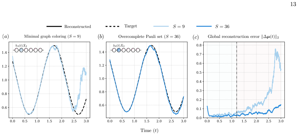
Summary. The manuscript develops a protocol for learning time-dependent, sparsely interacting Pauli Hamiltonians from ensemble-averaged continuous weak measurements. The key idea is to convert finite differences of monitored local Z expectation values into local linear inverse problems, whose size is controlled by the interaction degree rather than the total system size. The authors construct separable probe sets via graph coloring, prove that the number of global probe configurations is bounded by the active-neighborhood chromatic number times the maximum local neighborhood size, and state an error bound (Proposition 2) and a sample-complexity theorem (Theorem 1). Numerical simulations on TFIM-like chains with n up to 8 qubits show good reconstruction with an overcomplete Pauli-eigenstate ensemble over the chosen window, while the minimal graph-coloring ensemble is shown to lose stability at later times.
Significance. If the stated guarantees were fully a priori, the paper would be a substantial contribution to time-dependent Hamiltonian learning: the locality reduction to O(D)-sized inverse problems, the use of pure separable probes, and the explicit graph-coloring construction are valuable and experimentally relevant. The numerical experiments are extensive for a proof-of-concept study, and the code availability statement supports reproducibility. However, the central sample-complexity theorem is conditional on quantities that are not known before the experiment — most importantly the accumulated reconstruction error appearing in B_det and the data-dependent smallest singular value of the estimated reconstruction matrix — and the full-rank condition is not established beyond time t0. The numerical results even indicate that the advertised minimal probe ensemble violates this condition at later times. The framework is therefore promising, but the advertised guarantee is not yet closed.
major comments (3)
- [Section V, Eqs. (47)–(55), Theorem 1] The sample-complexity theorem is not a checkable a priori guarantee. B_det(t_k, Δt) in Eq. (53) contains ΔH_max(t_k), the supremum of the accumulated reconstruction error, so Eq. (48) is an implicit inequality for E_k = ||μhat(t_k)-μ(t_k)||_2. The condition in Eq. (54) and the denominator in Eq. (55) therefore depend on the very error the protocol is trying to bound. No discrete Grönwall step or smallness hypothesis is provided to close the recursion, and σ_min(Mhat) and the Lipschitz constant L in Eq. (A25) are also data- or unknown-Hamiltonian-dependent. The theorem is logically valid as a conditional statement, but as written it does not allow an experimenter to compute N_s from known inputs before running the protocol. I recommend either closing the recursion with explicit hypotheses on the coefficient magnitudes, the window length, and a certified conditioning bound, or reformulatin
- [Section IV and Proposition 2] The full-column-rank assumption on Mhat_loc_j(t_k) is only justified at the initial time. Section IV explicitly states that the construction guarantees solvability at t0, while later matrices are formed from the propagated state estimates in Eq. (33). Proposition 2 assumes full rank at t_k, but the protocol neither certifies nor preserves this property. Appendix B uses an SVD cutoff of 5×10^-3, and the numerical results in Section VI.b show the minimal graph-coloring ensemble (S=9) becoming unstable at later times, with the authors attributing this to dephasing making 'some local reconstruction matrices poorly conditioned.' Since Eq. (27) and the bound in Eq. (48) break down precisely in that regime, the theorem does not substantiate the advertised minimal-probe-set claim over the full reconstruction window. The authors should either prove a conditioning certificate for a chosen probe en
- [Section VI.c and Appendix B] The numerical validation of the sample-complexity scaling is useful but does not directly test Theorem 1. The fitted exponents α≈0.36–0.42 are compared with the conservative N_tot^{-1/2} sampling term, but the plotted quantity Err(T_sc) is not the bound in Eq. (48), and the dependence on σ_min(Mhat), Δt, and the Savitzky–Golay filter is not isolated. In addition, the theorem does not account for the filter or the SVD cutoff used in the implementation. Please clarify which aspects of the numerics are quantitative tests of the theorem and which are heuristic demonstrations of the pipeline, and either include the preprocessing effects in the bound or justify their neglect.
minor comments (4)
- [Section V heading] The heading contains a typo: 'PERFOMANCE' should be 'PERFORMANCE'.
- [Appendix B] The Savitzky–Golay window, the SVD cutoff, and the empirical prefactor η=0.1 in Δt_opt are numerical choices whose influence on the theoretical bounds is not discussed. This should be stated more explicitly so that the relation between the simulated pipeline and Proposition 2 is transparent.
- [Section III.B, Eq. (26)] The condition S ≥ |N(j)| is necessary but not sufficient for full column rank; the local probes must also provide linearly independent rows. This is implicit in the text, but stating it explicitly would prevent a misreading of the local identifiability condition.
- [Section V, Theorem 1] The theorem uses σ_min(Mhat) without an overbar to distinguish the data-dependent estimated-matrix value from a problem-level constant. Since this quantity enters the claimed trajectory bound, please clarify in the theorem statement that the condition and the N_s formula are functions of the realized state estimates.
Circularity Check
No significant circularity: the protocol inverts measured finite differences under explicit conditions; the ΔH_max-dependence in Theorem 1 is a conditional gap, not a definitional reduction.
full rationale
The core reconstruction step is a direct inversion of the linear response model, not a fitted quantity relabeled as a prediction. Equation (25) defines dΣ_j = M_loc_j μ_N(j) + O(Δt), and Eq. (27) estimates μ_N(j) by the Moore–Penrose inverse of M_loc_j applied to the measured finite differences. The matrices M_loc_j are built from the current state estimates and the known Pauli structure, so the estimate is obtained by inverting the same model that defines the data; this is the standard structure of a parameter-estimation protocol, not circular reasoning. The graph-coloring construction (Proposition 1) is an explicit construction: it prepares product states whose Pauli expectation values activate the local commutator columns, and its probe-count bound follows from the coloring and the local neighborhood size, not from the coefficients being learned. The main sample-complexity theorem is conditional rather than self-deriving. Theorem 1 assumes condition (54), ϵ > (√n/σ_min(Mhat)) B_det(t_k,Δt), where B_det in Eq. (53) contains ΔH_max(t_k), the accumulated Hamiltonian error. This does make the guarantee conditional on a quantity related to the very error being bounded, and the paper acknowledges this: "The condition in Eq. (54) states that the requested accuracy must be larger than the deterministic bias accumulated by the state update." But this is an uninstantiated hypothesis of an achievability statement, not an equation that defines the conclusion in terms of itself. The theorem is logically valid as a conditional; it is incomplete as a checkable a priori guarantee, which is a limitation of the error analysis rather than circularity. Numerical scaling exponents (α≈0.4, β) are fitted to the authors' simulations and are explicitly presented as observed behavior consistent with the theorem, not as inputs that produce the theorem. Self-citations appear only as background, static-HL context, or numerical simulation conventions (e.g., Refs. [10], [38], [55]); none is invoked as a uniqueness theorem or as the justification for the central inverse-problem reduction. The unproven full-rank condition at later times is a missing precondition, not a circular step. Hence no load-bearing circularity is present.
Axiom & Free-Parameter Ledger
free parameters (3)
- numerical time-step prefactor eta in Δt_opt scaling =
0.1
- SVD cutoff for pseudoinverse =
5e-3
- Savitzky-Golay filter window =
approximately 0.35 time units
axioms (7)
- domain assumption Hamiltonian has known sparse Pauli structure with unknown time-dependent coefficients (Eq. 1).
- domain assumption Continuous weak measurement backaction is described by the local dephasing master equation (Eq. 6) with known calibrated rates Γ_j.
- domain assumption Weak measurement records provide unbiased bounded estimates of Tr[Z_j ρ(t)] with Hoeffding-type concentration.
- domain assumption The effective generator is Lipschitz in trace norm along the relevant trajectories, with constant L, and the exact trajectory has uniformly bounded second derivative with constant C.
- ad hoc to paper All local reconstruction matrices M_loc_j(t_k) have full column rank at every reconstruction time.
- domain assumption Hamiltonian coefficients that commute with all monitored Z_j observables are either absent or known in advance.
- standard math Standard graph-coloring bound χ(G) ≤ D+1 and Hoeffding concentration, Hölder inequality, Moore-Penrose stability.
read the original abstract
Characterizing the Hamiltonian that a quantum processor actually implements is central to calibrating and validating current quantum hardware. Many devices, however, operate with generators that are time dependent by design. Here we develop a rigorous and experimentally friendly protocol for learning time-dependent many-body Hamiltonians from continuous weak measurement records. The key observation is that interaction sparsity reduces the global reconstruction to a set of local inverse problems, whose number is controlled by the interaction connectivity rather than by the system size. Pure separable probe states suffice to drive these inversions, and a graph-coloring construction embeds them into a small number of global product-state preparations. We derive explicit reconstruction-error bounds and a sample-complexity theorem that cleanly separates the finite-sampling statistical noise from the deterministic bias of the iterative state update, and we validate the protocol on time-dependent spin chains with up to $n=8$ qubits. Beyond these results, our analysis provides a rigorous foundation for time-dependent Hamiltonian learning from continuous monitoring in many-body systems, establishing a framework that extends naturally to many platforms and probe ensembles.
Figures




Reference graph
Works this paper leans on
-
[1]
Preskill, Quantum computing in the nisq era and be- yond, Quantum2, 79 (2018)
J. Preskill, Quantum computing in the nisq era and be- yond, Quantum2, 79 (2018)
2018
-
[2]
I. M. Georgescu, S. Ashhab, and F. Nori, Quantum sim- ulation, Reviews of Modern Physics86, 153 (2014)
2014
-
[3]
S. Ebadi, T. T. Wang, H. Levine, A. Keesling, G. Se- meghini, A. Omran, D. Bluvstein, R. Samajdar, H. Pich- ler, W. W. Ho, S. Choi, S. Sachdev, M. Greiner, V. Vuleti´ c, and M. D. Lukin, Quantum phases of matter on a 256-atom programmable quantum simulator, Nature 595, 227 (2021), arXiv:2012.12281 [quant-ph]
Pith/arXiv arXiv 2021
-
[4]
Wiebe, C
N. Wiebe, C. Granade, C. Ferrie, and D. G. Cory, Hamiltonian learning and certification using quantum re- sources, Phys. Rev. Lett.112, 190501 (2014)
2014
-
[5]
Eisert, D
J. Eisert, D. Hangleiter, N. Walk, I. Roth, D. Markham, R. Parekh, U. Chabaud, and E. Kashefi, Quantum cer- tification and benchmarking, Nature Reviews Physics2, 382 (2020)
2020
-
[6]
C. E. Granade, C. Ferrie, N. Wiebe, and D. G. Cory, Ro- bust online hamiltonian learning, New Journal of Physics 14, 103013 (2012)
2012
-
[7]
Wiebe, C
N. Wiebe, C. Granade, C. Ferrie, and D. Cory, Quantum hamiltonian learning using imperfect quantum resources, Phys. Rev. A89, 042314 (2014)
2014
-
[8]
K. Siva, G. Koolstra, J. Steinmetz, W. P. Livingston, D. Das, L. Chen, J. Kreikebaum, N. Stevenson, C. J¨ unger, D. Santiago, I. Siddiqi, and A. Jordan, Time- dependent hamiltonian reconstruction using continuous weak measurements, PRX Quantum4, 040324 (2023)
2023
-
[9]
A. Gu, L. Cincio, and P. J. Coles, Practical hamiltonian learning with unitary dynamics and gibbs states, Nature 16 Communications15, 312 (2024)
2024
-
[10]
G. Franceschetto, E. Pagliaro, L. Pereira, L. Zambrano, and A. Ac ´ ın, Hamiltonian learning via quantum zeno ef- fect (2025), arXiv:2509.15713 [quant-ph]
arXiv 2025
-
[11]
Huang, Y
H.-Y. Huang, Y. Tong, D. Fang, and Y. Su, Learning many-body hamiltonians with heisenberg-limited scaling, Physical Review Letters130, 200403 (2023)
2023
-
[12]
Wang, D.-L
S.-T. Wang, D.-L. Deng, and L.-M. Duan, Hamiltonian tomography for quantum many-body systems with ar- bitrary couplings, New Journal of Physics17, 093017 (2015)
2015
-
[13]
J. Haah, R. Kothari, and E. Tang, Learning quan- tum hamiltonians from high-temperature gibbs states and real-time evolutions, Nature Physics20, 1027–1031 (2024)
2024
-
[14]
W. Yu, J. Sun, Z. Han, and X. Yuan, Robust and efficient hamiltonian learning, Quantum7, 1045 (2023)
2023
-
[15]
D. Stilck Fran¸ ca, L. A. Markovich, V. V. Dobrovitski, A. H. Werner, and J. Borregaard, Efficient and robust estimation of many-qubit hamiltonians, Nature Commu- nications15, 10.1038/s41467-023-44012-5 (2024)
-
[16]
Heightman, E
T. Heightman, E. Jiang, and A. Ac ´ ın, Solving the quan- tum many-body hamiltonian learning problem with neu- ral differential equations, Quantum Science and Technol- ogy10, 045072 (2025)
2025
-
[17]
Baran and T
B. Baran and T. Heightman, Heisenberg-limited quan- tum hamiltonian learning via randomly spread product- states (2025)
2025
-
[18]
L. Pastori, T. Olsacher, C. Kokail, and P. Zoller, Charac- terization and verification of trotterized digital quantum simulation via hamiltonian and liouvillian learning, PRX Quantum3, 030324 (2022), arXiv:2203.15846 [quant-ph]
Pith/arXiv arXiv 2022
-
[19]
T. Olsacher, T. Kraft, C. Kokail, B. Kraus, and P. Zoller, Hamiltonian and liouvillian learning in weakly-dissipative quantum many-body systems, Quan- tum Science and Technology10, 015065 (2025), arXiv:2405.06768 [quant-ph]
Pith/arXiv arXiv 2025
-
[20]
Bairey, I
E. Bairey, I. Arad, and N. H. Lindner, Learning a local hamiltonian from local measurements, Phys. Rev. Lett. 122, 020504 (2019)
2019
-
[21]
D. Hangleiter, I. Roth, J. Fuksa, J. Eisert, and P. Roushan, Robustly learning the hamiltonian dynamics of a superconducting quantum processor, Nature Com- munications15, 10.1038/s41467-024-52629-3 (2024)
-
[22]
S.-A. Guo, Y.-K. Wu, J. Ye, L. Zhang, Y. Wang, W.-Q. Lian, R. Yao, Y.-L. Xu, C. Zhang, Y.-Z. Xu, B.-X. Qi, P.-Y. Hou, L. He, Z.-C. Zhou, and L.-M. Duan, Hamilto- nian learning for 300 trapped ion qubits with long-range couplings, Science Advances11, 10.1126/sciadv.adt4713 (2025)
-
[23]
J. M. Chow, L. DiCarlo, J. M. Gambetta, F. Motzoi, L. Frunzio, S. M. Girvin, and R. J. Schoelkopf, Optimized driving of superconducting artificial atoms for improved single-qubit gates, Physical Review A82, 040305 (2010)
2010
-
[24]
Y. Chen, C. Neill, P. Roushan, N. Leung, M. Fang, R. Barends, J. Kelly, B. Campbell, Z. Chen, B. Chiaro, A. Dunsworth, E. Jeffrey, A. Megrant, J. Y. Mu- tus, P. J. J. O’Malley, C. M. Quintana, D. Sank, A. Vainsencher, J. Wenner, T. C. White, M. R. Geller, A. N. Cleland, and J. M. Martinis, Qubit architecture with high coherence and fast tunable coupling, ...
2014
-
[25]
E. A. Sete, N. Didier, A. Q. Chen, S. Kulshreshtha, R. Manenti, and S. Poletto, Parametric-resonance entan- gling gates with a tunable coupler, Physical Review Ap- plied16, 024050 (2021)
2021
-
[26]
Randall, C
J. Randall, C. E. Bradley, F. V. van der Gron- den, A. Galicia, M. H. Abobeih, M. Markham, D. J. Twitchen, F. Machado, N. Y. Yao, and T. H. Taminiau, Many-body–localized discrete time crystal with a pro- grammable spin-based quantum simulator, Science374, 1474 (2021)
2021
-
[27]
D. Stilck Fran¸ ca, T. M¨ obus, C. Rouz´ e, and A. H. Werner, Learning and certification of local time-dependent quantum dynamics and noise (2025), arXiv:2510.08500 [quant-ph]
arXiv 2025
-
[28]
Jacobs and D
K. Jacobs and D. A. Steck, A straightforward introduc- tion to continuous quantum measurement, Contempo- rary Physics47, 279 (2006)
2006
-
[29]
K. W. Murch, S. J. Weber, C. Macklin, and I. Siddiqi, Observing single quantum trajectories of a superconduct- ing quantum bit, Nature502, 211 (2013)
2013
-
[30]
S. J. Weber, K. W. Murch, M. E. Kimchi-Schwartz, N. Roch, and I. Siddiqi, Quantum trajectories of super- conducting qubits, Comptes Rendus Physique17, 766 (2016)
2016
-
[31]
Hacohen-Gourgy and L
S. Hacohen-Gourgy and L. S. Martin, Continuous mea- surements for control of superconducting quantum cir- cuits, Advances in Physics: X5, 1813626 (2020)
2020
-
[32]
Y. Pan, J. Zhang, E. Cohen, C.-W. Wu, P.-X. Chen, and N. Davidson, Weak-to-strong transition of quantum measurement in a trapped-ion system, Nature Physics 16, 1206 (2020)
2020
-
[33]
G. A. Smith, S. Chaudhury, A. Silberfarb, I. H. Deutsch, and P. S. Jessen, Continuous weak measurement and non- linear dynamics in a cold spin ensemble, Physical Review Letters93, 163602 (2004)
2004
-
[34]
G. A. Smith, A. Silberfarb, I. H. Deutsch, and P. S. Jessen, Efficient quantum state estimation by continu- ous weak measurement and dynamical control, Physical Review Letters97, 180403 (2006)
2006
-
[35]
K. W. Murch, K. L. Moore, S. Gupta, and D. M. Stamper-Kurn, Observation of quantum-measurement backaction with an ultracold atomic gas, Nature Physics 4, 561 (2008)
2008
-
[36]
Altuntas and I
E. Altuntas and I. B. Spielman, Weak-measurement- induced heating in bose-einstein condensates, Physical Review Research5, 023185 (2023)
2023
-
[37]
Rossi, D
M. Rossi, D. Mason, J. Chen, and A. Schliesser, Observ- ing and verifying the quantum trajectory of a mechanical resonator, Physical Review Letters123, 163601 (2019)
2019
-
[38]
G. Franceschetto, P. Mujal, and R. Mart ´ ınez-Pe˜ na, Measurement-enabled online quantum processing with amplitude encoding (2026), arXiv:2606.18991 [quant-ph]
Pith/arXiv arXiv 2026
-
[39]
Hatridge, S
M. Hatridge, S. Shankar, M. Mirrahimi, F. Schackert, K. Geerlings, T. Brecht, K. M. Sliwa, B. Abdo, L. Frun- zio, S. M. Girvin, R. J. Schoelkopf, and M. H. Devoret, Quantum back-action of an individual variable-strength measurement, Science339, 178 (2013)
2013
-
[40]
Mujal, R
P. Mujal, R. Mart ´ ınez-Pe˜ na, G. L. Giorgi, M. C. Soriano, and R. Zambrini, Time-series quantum reservoir comput- ing with weak and projective measurements, npj Quan- tum Information9, 16 (2023)
2023
-
[41]
Diestel,Graph Theory, 5th ed
R. Diestel,Graph Theory, 5th ed. (Springer, 2017)
2017
-
[42]
Ben-Israel and T
A. Ben-Israel and T. N. E. Greville,Generalized Inverses: Theory and Applications, 2nd ed. (Springer, 2003)
2003
-
[43]
G. Vidal, Efficient simulation of one-dimensional quan- tum many-body systems, Physical Review Letters93, 17 040502 (2004), arXiv:quant-ph/0310089
Pith/arXiv arXiv 2004
-
[44]
J. Haegeman, C. Lubich, I. Oseledets, B. Vandereycken, and F. Verstraete, Unifying time evolution and optimiza- tion with matrix product states, Physical Review B94, 165116 (2016), arXiv:1408.5056 [quant-ph]
Pith/arXiv arXiv 2016
-
[45]
J. Hauschild and F. Pollmann, Efficient numerical sim- ulations with tensor networks: Tensor network python (tenpy), SciPost Physics Lecture Notes , 005 (2018), arXiv:1805.00055 [cond-mat.str-el]
Pith/arXiv arXiv 2018
-
[46]
A. Klappenecker and M. R¨ otteler, Mutually unbiased bases are complex projective 2-designs, inProceedings of the IEEE International Symposium on Information The- ory(2005) pp. 1740–1744, arXiv:quant-ph/0502031
Pith/arXiv arXiv 2005
-
[47]
C. Dankert, R. Cleve, J. Emerson, and E. Livine, Ex- act and approximate unitary 2-designs and their applica- tion to fidelity estimation, Physical Review A80, 012304 (2009), arXiv:quant-ph/0606161
Pith/arXiv arXiv 2009
- [48]
-
[49]
H. Zhu, Mutually unbiased bases as minimal clifford co- variant 2-designs, Physical Review A91, 060301 (2015), arXiv:1505.01123 [quant-ph]
Pith/arXiv arXiv 2015
-
[50]
G. Lami, T. Haug, and J. De Nardis, Quantum state de- signs with clifford-enhanced matrix product states, PRX Quantum6, 010345 (2025), arXiv:2404.18751 [quant-ph]
Pith/arXiv arXiv 2025
-
[51]
Arute, K
F. Arute, K. Arya, R. Babbush, andet al., Quantum supremacy using a programmable superconducting pro- cessor, Nature574, 505 (2019)
2019
-
[52]
C. Chamberland, G. Zhu, T. J. Yoder, J. B. Hertzberg, and A. W. Cross, Topological and subsystem codes on low-degree graphs with flag qubits, Physical Review X 10, 011022 (2020), arXiv:1907.09528 [quant-ph]
Pith/arXiv arXiv 2020
-
[53]
Browaeys and T
A. Browaeys and T. Lahaye, Many-body physics with in- dividually controlled rydberg atoms, Nature Physics16, 132 (2020). [54]https://github.com/jesusjimrod/TDHL.git
2020
-
[55]
G. Franceschetto, M. P lodzie´ n, M. Lewenstein, A. Ac ´ ın, and P. Mujal, Harnessing quantum backaction for time- series processing, Physical Review X16, 10.1103/j7f9- hfsj (2026). Appendix A: Details of the reconstruction-error bound This appendix provides the technical derivation of Proposition 2 and Theorem 1. We first collect the norm and concentrati...
-
[56]
Definition 4(Induced matrix norm).Let∥ · ∥be a norm on a vector space
Norms and concentration tools We first recall the norm conventions used in the derivation. Definition 4(Induced matrix norm).Let∥ · ∥be a norm on a vector space. The matrix norm induced by∥ · ∥is defined as ∥A∥:= sup x̸=0 ∥Ax∥ ∥x∥ = sup ∥x∥=1 ∥Ax∥.(A1) In particular, the norm induced by the Euclidean norm is the spectral norm, which coincides with the Sch...
-
[57]
Fix a monitored sitejand a recon- struction timet k
Concentration of the finite-difference data vector We derive the concentration bound for the empirical finite-difference vectors. Fix a monitored sitejand a recon- struction timet k. For this site, the stacked record over theSprobe configurations is zj(tk) = z(1) j (tk), . . . , z(S) j (tk) T , dΣ j(tk) = zj(tk+1)−z j(tk) ∆t .(A8) The corresponding empiri...
-
[58]
Fix a monitored sitejand a reconstruction timet k
Perturbation of the reconstruction matrices We now derive the deterministic matrix-perturbation bound used in Proposition 2. Fix a monitored sitejand a reconstruction timet k. We suppress the explicit time dependence and write ∆M j = ˆMj −M j, whereM j =M loc j (tk), ˆMj = ˆMloc j (tk), andρ s =ρ s(tk). The entries of ∆M j are (∆Mj)sm =−iTr([Z j, Wm](ˆρs ...
-
[59]
KD+MCg69HFArnNyc+UTgfZMhSN0=
Global reconstruction bound and proof of Theorem 1 This section analyzes the asymptotic scaling of the full protocol and justifies the global reconstruction bound used in the main text. Let∥∆µ(t k)∥denote the norm of the difference between the reconstructed and true coefficients of the global Hamiltonian, and∥∆µ j(tk)∥the corresponding norm restricted to ...
discussion (0)
Sign in with ORCID, Apple, or X to comment. Anyone can read and Pith papers without signing in.