CT-OT Flow: Estimating Continuous-Time Dynamics from Discrete Temporal Snapshots
Pith reviewed 2026-05-25 08:33 UTC · model grok-4.3
The pith
CT-OT Flow recovers continuous-time dynamics from aggregated snapshots by inferring time labels via partial optimal transport and smoothing distributions to train ODE models.
A machine-rendered reading of the paper's core claim, the machinery that carries it, and where it could break.
Core claim
CT-OT Flow is a two-stage framework that infers high-resolution time labels by aligning neighboring intervals via partial optimal transport and reconstructs a continuous-time data distribution through temporal kernel smoothing, from which pairs of nearby times are sampled to train standard ODE/SDE models, explicitly accounting for snapshot aggregation and time-label uncertainty while using screening and mini-batch accelerations for scalability.
What carries the argument
Two-stage process of partial optimal transport alignment for time-label inference followed by temporal kernel smoothing for distribution reconstruction.
If this is right
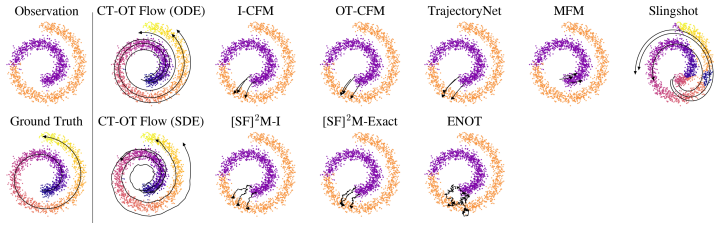
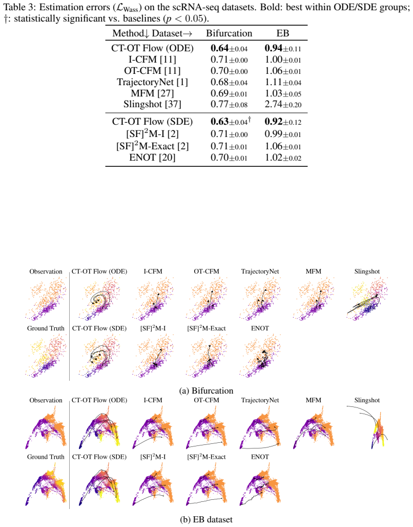
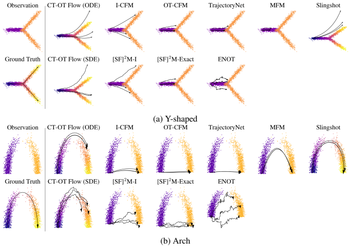
- Distributional and trajectory errors decrease relative to OT-CFM, [SF]²M, TrajectoryNet, MFM, and ENOT on synthetic benchmarks and on scRNA-seq and typhoon-track data.
- The framework scales to large datasets through screening and mini-batch partial optimal transport.
- Explicit modeling of aggregation and time uncertainty allows training of continuous-time models without direct trajectory observations.
- Sampled nearby-time pairs from the smoothed distribution serve as training data for standard ODE or SDE solvers.
Where Pith is reading between the lines
- The same alignment-plus-smoothing pattern could be applied to other snapshot-only domains such as video-frame sequences or financial tick data.
- If the inferred labels prove reliable, downstream tasks such as estimating transition rates between states become feasible on the same datasets.
- Direct comparison against known continuous paths on additional controlled simulations would provide a clear test of the label-recovery step.
Load-bearing premise
Partial optimal transport alignment of neighboring intervals can reliably recover accurate high-resolution time labels from aggregated snapshots that have noisy or uncertain timestamps.
What would settle it
On a synthetic dataset where ground-truth continuous trajectories and exact times are known, the time labels produced by the partial optimal transport step would deviate substantially from the true times.
Figures




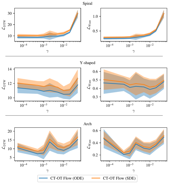




read the original abstract
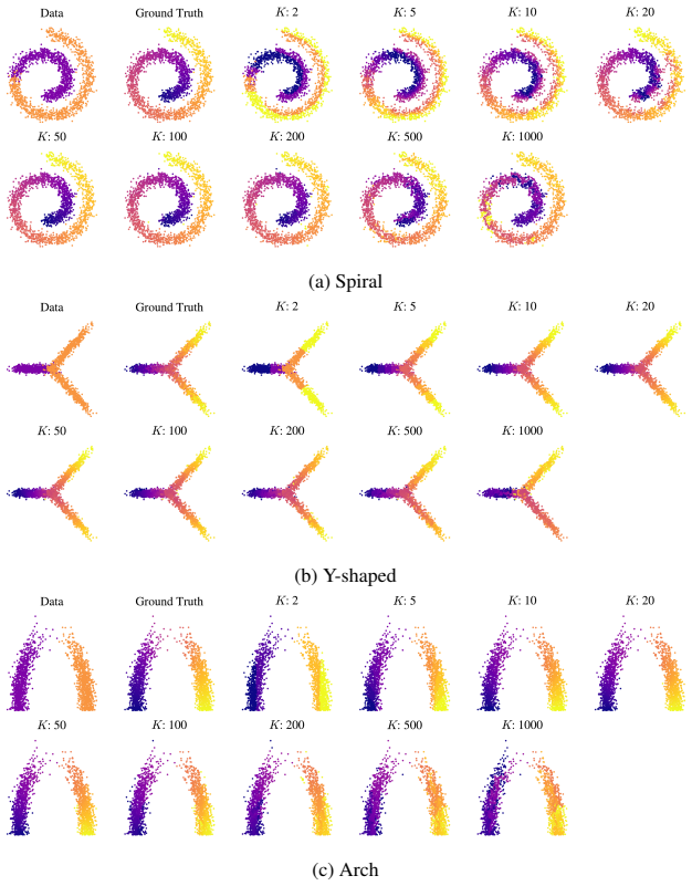
In many real-world settings--e.g., single-cell RNA sequencing, mobility sensing, and environmental monitoring--data are observed only as temporally aggregated snapshots collected over finite time windows, often with noisy or uncertain timestamps, and without access to continuous trajectories. We study the problem of estimating continuous-time dynamics from such snapshots. We present Continuous-Time Optimal Transport Flow (CT-OT Flow), a two-stage framework that (i) infers high-resolution time labels by aligning neighboring intervals via partial optimal transport (POT) and (ii) reconstructs a continuous-time data distribution through temporal kernel smoothing, from which we sample pairs of nearby times to train standard ODE/SDE models. Our formulation explicitly accounts for snapshot aggregation and time-label uncertainty and uses practical accelerations (screening and mini-batch POT), making it applicable to large datasets. Across synthetic benchmarks and two real datasets (scRNA-seq and typhoon tracks), CT-OT Flow reduces distributional and trajectory errors compared with OT-CFM, [SF]\(^{2}\)M, TrajectoryNet, MFM, and ENOT.
Editorial analysis
A structured set of objections, weighed in public.
Referee Report
Summary. The paper proposes CT-OT Flow, a two-stage method for recovering continuous-time dynamics from temporally aggregated snapshots that may have noisy or uncertain timestamps. Stage (i) aligns neighboring intervals with partial optimal transport (POT) to infer high-resolution time labels; stage (ii) applies temporal kernel smoothing to reconstruct a continuous distribution from which nearby-time pairs are sampled to train standard ODE/SDE models. Practical accelerations (screening, mini-batch POT) are included. The central empirical claim is that the method yields lower distributional and trajectory errors than OT-CFM, [SF]²M, TrajectoryNet, MFM, and ENOT on synthetic benchmarks plus scRNA-seq and typhoon-track data.
Significance. If the POT-based label recovery proves reliable under realistic noise, the framework would supply a practical route to continuous-time modeling in snapshot-only regimes such as single-cell genomics and environmental sensing. The explicit treatment of aggregation and uncertainty, together with the reported accelerations for large data, are constructive features. The absence of isolated diagnostics for the label-recovery step, however, leaves the source of the reported gains unclear.
major comments (3)
- [Abstract, §3] Abstract and §3 (first stage): the performance claim that CT-OT Flow reduces distributional/trajectory error relative to the listed baselines rests on the accuracy of the inferred high-resolution time labels produced by partial OT alignment. No diagnostic is reported that measures label-recovery error versus ground truth on synthetic data whose timestamp noise matches the regimes of the scRNA-seq or typhoon datasets; without this isolation it is impossible to determine whether downstream gains arise from the claimed continuous-time recovery or from smoothing/model choice alone.
- [§5] §5 (experiments): the abstract states that error reductions are observed, yet the provided text supplies neither error bars, ablation studies on the POT component, nor analysis of failure modes when alignment quality degrades. These omissions make the robustness of the cross-method comparisons difficult to assess.
- [§4] §4 (model training): the formulation is said to 'explicitly account for snapshot aggregation and time-label uncertainty,' but the manuscript does not quantify how residual label error propagates into the kernel-smoothed distribution or the subsequent ODE/SDE training objective.
minor comments (2)
- [Abstract] The acronym [SF]²M should be expanded on first use or a reference supplied.
- [§3] Notation distinguishing the partial OT cost from the subsequent kernel smoothing bandwidth would improve readability.
Simulated Author's Rebuttal
We thank the referee for the detailed and constructive feedback. The comments highlight the need for clearer isolation of the label-recovery stage and additional robustness checks. We address each major comment below and will incorporate the suggested diagnostics and analyses in a revised manuscript.
read point-by-point responses
-
Referee: [Abstract, §3] Abstract and §3 (first stage): the performance claim that CT-OT Flow reduces distributional/trajectory error relative to the listed baselines rests on the accuracy of the inferred high-resolution time labels produced by partial OT alignment. No diagnostic is reported that measures label-recovery error versus ground truth on synthetic data whose timestamp noise matches the regimes of the scRNA-seq or typhoon datasets; without this isolation it is impossible to determine whether downstream gains arise from the claimed continuous-time recovery or from smoothing/model choice alone.
Authors: We agree that an isolated evaluation of the partial-OT label-recovery step would strengthen the paper. On the synthetic benchmarks already used in the manuscript we possess ground-truth timestamps; we will add a new subsection (or appendix) that reports label-recovery error (e.g., mean absolute deviation and Wasserstein distance between recovered and true time labels) under controlled timestamp noise levels calibrated to the aggregation windows observed in the scRNA-seq and typhoon data. This will allow readers to separate the contribution of the alignment stage from the subsequent kernel-smoothing and flow training. revision: yes
-
Referee: [§5] §5 (experiments): the abstract states that error reductions are observed, yet the provided text supplies neither error bars, ablation studies on the POT component, nor analysis of failure modes when alignment quality degrades. These omissions make the robustness of the cross-method comparisons difficult to assess.
Authors: We will revise §5 to include (i) error bars computed over at least five independent random seeds for all reported metrics, (ii) an ablation that disables the POT alignment stage (replacing it with uniform or noisy time labels) while keeping the kernel-smoothing and ODE/SDE training identical, and (iii) a short discussion of failure regimes, e.g., when neighboring snapshot intervals become too distant for reliable partial transport or when label noise exceeds the bandwidth of the temporal kernel. These additions will make the empirical claims more transparent. revision: yes
-
Referee: [§4] §4 (model training): the formulation is said to 'explicitly account for snapshot aggregation and time-label uncertainty,' but the manuscript does not quantify how residual label error propagates into the kernel-smoothed distribution or the subsequent ODE/SDE training objective.
Authors: We acknowledge that a quantitative propagation analysis is currently missing. In the revision we will add a sensitivity study (new paragraph in §4 or dedicated appendix) that injects controlled label perturbations into the recovered times, recomputes the kernel-smoothed densities, and measures the resulting change in the flow-matching loss and downstream trajectory error. This will provide an empirical bound on how label-recovery inaccuracies affect the final model. revision: yes
Circularity Check
No circularity; method uses external POT alignment and standard ODE/SDE training against independent baselines.
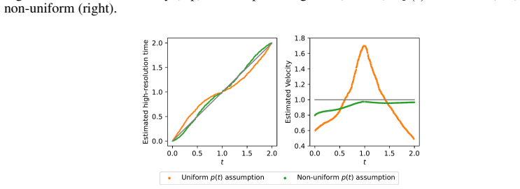
full rationale
The described framework infers time labels via partial optimal transport (an external technique), applies temporal kernel smoothing, and trains standard ODE/SDE models. Performance is evaluated via direct comparison to external methods (OT-CFM, TrajectoryNet, MFM, ENOT, etc.) on synthetic and real data. No self-definitional reductions, fitted inputs renamed as predictions, or load-bearing self-citations appear in the provided text. The derivation chain remains independent of its own outputs.
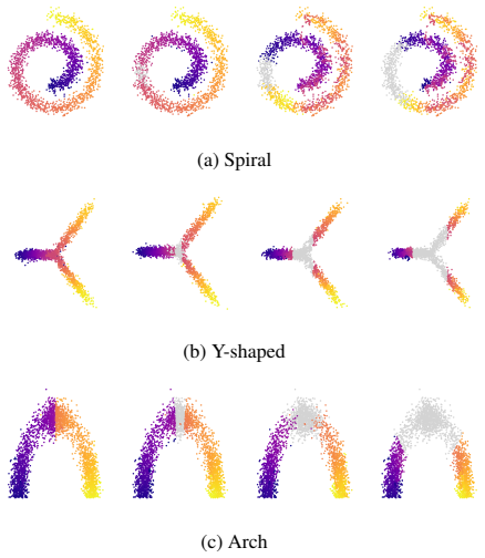
Axiom & Free-Parameter Ledger
axioms (1)
- domain assumption Data are observed only as temporally aggregated snapshots collected over finite time windows, often with noisy or uncertain timestamps.
Lean theorems connected to this paper
-
IndisputableMonolith/Cost/FunctionalEquation.leanwashburn_uniqueness_aczel unclear?
unclearRelation between the paper passage and the cited Recognition theorem.
CT-OT Flow employs partial optimal transport (POT) to infer high-resolution time labels... kernel-based smoothing approach... ˜p_t(x) = 1/Z_kernel(t) Σ k(t, ˜t^(i)) δ_x^(i)(x)
-
IndisputableMonolith/Foundation/RealityFromDistinction.leanreality_from_one_distinction unclear?
unclearRelation between the paper passage and the cited Recognition theorem.
We assume that the underlying distribution p_t(x) is continuous in t... lim Δt→0 p[t,t+Δt](x) = p_t(x)
What do these tags mean?
- matches
- The paper's claim is directly supported by a theorem in the formal canon.
- supports
- The theorem supports part of the paper's argument, but the paper may add assumptions or extra steps.
- extends
- The paper goes beyond the formal theorem; the theorem is a base layer rather than the whole result.
- uses
- The paper appears to rely on the theorem as machinery.
- contradicts
- The paper's claim conflicts with a theorem or certificate in the canon.
- unclear
- Pith found a possible connection, but the passage is too broad, indirect, or ambiguous to say the theorem truly supports the claim.
Reference graph
Works this paper leans on
-
[1]
Trajecto- rynet: A dynamic optimal transport network for modeling cellular dynamics
Alexander Tong, Jessie Huang, Guy Wolf, David van Dijk, and Smita Krishnaswamy. Trajecto- rynet: A dynamic optimal transport network for modeling cellular dynamics. InProceedings of the 37th International Conference on Machine Learning, 2020
work page 2020
-
[2]
Simulation-free Schrödinger bridges via score and flow matching
Alexander Y Tong, Nikolay Malkin, Kilian Fatras, Lazar Atanackovic, Yanlei Zhang, Guillaume Huguet, Guy Wolf, and Yoshua Bengio. Simulation-free Schrödinger bridges via score and flow matching. InInternational Conference on Artificial Intelligence and Statistics, pages 1279–1287. PMLR, 2024
work page 2024
-
[3]
Haifeng Niu and Elisabete A Silva. Understanding temporal and spatial patterns of urban activi- ties across demographic groups through geotagged social media data.Computers, Environment and Urban Systems, 100:101934, 2023. 12
work page 2023
-
[4]
Charlotte Bunne, Stefan G Stark, Gabriele Gut, Jacobo Sarabia Del Castillo, Mitch Levesque, Kjong-Van Lehmann, Lucas Pelkmans, Andreas Krause, and Gunnar Rätsch. Learning single- cell perturbation responses using neural optimal transport.Nature Methods, 20(11):1759–1768, 2023
work page 2023
-
[5]
Grace XY Zheng, Jessica M Terry, Phillip Belgrader, Paul Ryvkin, Zachary W Bent, Ryan Wilson, Solongo B Ziraldo, Tobias D Wheeler, Geoff P McDermott, Junjie Zhu, et al. Massively parallel digital transcriptional profiling of single cells.Nature Communications, 8(1):14049, 2017
work page 2017
-
[6]
Rna velocity of single cells.Nature, 560(7719):494–498, 2018
Gioele La Manno, Ruslan Soldatov, Amit Zeisel, Emelie Braun, Hannah Hochgerner, Viktor Petukhov, Katja Lidschreiber, Maria E Kastriti, Peter Lönnerberg, Alessandro Furlan, et al. Rna velocity of single cells.Nature, 560(7719):494–498, 2018
work page 2018
-
[7]
Urban computing: Concepts, method- ologies, and applications.ACM Trans
Yu Zheng, Licia Capra, Ouri Wolfson, and Hai Yang. Urban computing: Concepts, method- ologies, and applications.ACM Trans. Intell. Syst. Technol., 5(3), September 2014. ISSN 2157-6904. doi: 10.1145/2629592
-
[8]
Wireless sensor network survey
Jennifer Yick, Biswanath Mukherjee, and Dipak Ghosal. Wireless sensor network survey. Computer Networks, 52(12):2292–2330, 2008
work page 2008
-
[9]
Ricky T. Q. Chen, Yulia Rubanova, Jesse Bettencourt, and David K Duvenaud. Neural ordinary differential equations. In S. Bengio, H. Wallach, H. Larochelle, K. Grauman, N. Cesa-Bianchi, and R. Garnett, editors,Advances in Neural Information Processing Systems, volume 31. Curran Associates, Inc., 2018
work page 2018
-
[10]
Christian Léonard. A survey of the Schrödinger problem and some of its connections with optimal transport.arXiv preprint arXiv:1308.0215, 2013
-
[11]
Alexander Tong, Kilian FATRAS, Nikolay Malkin, Guillaume Huguet, Yanlei Zhang, Jarrid Rector-Brooks, Guy Wolf, and Yoshua Bengio. Improving and generalizing flow-based genera- tive models with minibatch optimal transport.Transactions on Machine Learning Research, 2024
work page 2024
-
[12]
Embryoid body data for PHATE.Mendeley Data, 1, 2018
Kevin Moon. Embryoid body data for PHATE.Mendeley Data, 1, 2018
work page 2018
-
[13]
Spot: sliced partial optimal transport.ACM Trans
Nicolas Bonneel and David Coeurjolly. Spot: sliced partial optimal transport.ACM Trans. Graph., 38(4), July 2019. ISSN 0730-0301. doi: 10.1145/3306346.3323021
-
[14]
Alessio Figalli. The optimal partial transport problem.Archive for Rational Mechanics and Analysis, 195(2):533–560, 2010
work page 2010
-
[15]
Chen, Aviv Regev, and Romain Lopez
Martin Rohbeck, Charlotte Bunne, Edward De Brouwer, Jan-Christian Huetter, Anne Biton, Kelvin Y . Chen, Aviv Regev, and Romain Lopez. Modeling complex system dynamics with flow matching across time and conditions. InThe Thirteenth International Conference on Learning Representations, 2025
work page 2025
-
[16]
Flow match- ing for generative modeling
Yaron Lipman, Ricky TQ Chen, Heli Ben-Hamu, Maximilian Nickel, and Matt Le. Flow match- ing for generative modeling. In11th International Conference on Learning Representations, 2023
work page 2023
-
[17]
Flow straight and fast: Learning to generate and transfer data with rectified flow
Xingchao Liu, Chengyue Gong, and Qiang Liu. Flow straight and fast: Learning to generate and transfer data with rectified flow. In11th International Conference on Learning Representations, 2023
work page 2023
-
[18]
Light Schrödinger bridge.arXiv preprint arXiv:2310.01174, 2023
Alexander Korotin, Nikita Gushchin, and Evgeny Burnaev. Light Schrödinger bridge.arXiv preprint arXiv:2310.01174, 2023
-
[19]
Takeshi Koshizuka and Issei Sato. Neural lagrangian Schrödinger bridge: Diffusion modeling for population dynamics.arXiv preprint arXiv:2204.04853, 2022
-
[20]
Nikita Gushchin, Alexander Kolesov, Alexander Korotin, Dmitry P Vetrov, and Evgeny Burnaev. Entropic neural optimal transport via diffusion processes.Advances in Neural Information Processing Systems, 36, 2024. 13
work page 2024
-
[21]
Dominik Klein, Théo Uscidda, Fabian Theis, and Marco Cuturi. GENOT: Entropic (Gromov) Wasserstein flow matching with applications to single-cell genomics.Advances in Neural Information Processing Systems, 37:103897–103944, 2024
work page 2024
-
[22]
Score-based generative modeling through stochastic differential equations
Yang Song, Jascha Sohl-Dickstein, Diederik P Kingma, Abhishek Kumar, Stefano Ermon, and Ben Poole. Score-based generative modeling through stochastic differential equations. In International Conference on Learning Representations, 2021
work page 2021
-
[23]
Action matching: Learning stochastic dynamics from samples
Kirill Neklyudov, Rob Brekelmans, Daniel Severo, and Alireza Makhzani. Action matching: Learning stochastic dynamics from samples. InInternational conference on machine learning, pages 25858–25889. PMLR, 2023
work page 2023
-
[24]
Deep multi-marginal momentum Schrödinger bridge
Tianrong Chen, Guan-horng Liu, Molei Tao, and Evangelos A Theodorou. Deep multi-marginal momentum Schrödinger bridge. InProceedings of the 37th International Conference on Neural Information Processing Systems, pages 57058–57086, 2023
work page 2023
-
[25]
Justin Lee, Behnaz Moradijamei, and Heman Shakeri. Multi-marginal stochastic flow matching for high-dimensional snapshot data at irregular time points.arXiv preprint arXiv:2508.04351, 2025
-
[26]
Efficient trajectory inference in wasserstein space using consecutive averaging
Amartya Banerjee, Harlin Lee, Nir Sharon, and Caroline Moosmüller. Efficient trajectory inference in wasserstein space using consecutive averaging. InInternational Conference on Artificial Intelligence and Statistics, 2025
work page 2025
-
[27]
Kacper Kapusniak, Peter Potaptchik, Teodora Reu, Leo Zhang, Alexander Tong, Michael Bronstein, Avishek Joey Bose, and Francesco Di Giovanni. Metric flow matching for smooth interpolations on the data manifold.arXiv preprint arXiv:2405.14780, 2024
-
[28]
Flow matching on general geometries.arXiv preprint arXiv:2302.03660, 2023
Ricky TQ Chen and Yaron Lipman. Flow matching on general geometries.arXiv preprint arXiv:2302.03660, 2023
-
[29]
Gabriel Peyré, Marco Cuturi, et al. Computational optimal transport: With applications to data science.Foundations and Trends® in Machine Learning, 11(5-6):355–607, 2019
work page 2019
-
[30]
Sinkhorn distances: Lightspeed computation of optimal transport
Marco Cuturi. Sinkhorn distances: Lightspeed computation of optimal transport. In C.J. Burges, L. Bottou, M. Welling, Z. Ghahramani, and K.Q. Weinberger, editors,Advances in Neural Information Processing Systems, volume 26. Curran Associates, Inc., 2013
work page 2013
-
[31]
V olker Bergen, Marius Lange, Stefan Peidli, F. Alexander Wolf, and Fabian J. Theis. Generaliz- ing rna velocity to transient cell states through dynamical modeling.Nature Biotechnology, 38 (12):1408–1414, August 2020. ISSN 1546-1696. doi: 10.1038/s41587-020-0591-3
-
[32]
Cole Trapnell, Davide Cacchiarelli, Jonna Grimsby, Prapti Pokharel, Shuqiang Li, Michael Morse, Niall J Lennon, Kenneth J Livak, Tarjei S Mikkelsen, and John L Rinn. The dynamics and regulators of cell fate decisions are revealed by pseudotemporal ordering of single cells. Nature Biotechnology, 32(4):381–386, 2014
work page 2014
-
[33]
Xiaojie Qiu, Qi Mao, Ying Tang, Li Wang, Raghav Chawla, Hannah A Pliner, and Cole Trapnell. Reversed graph embedding resolves complex single-cell trajectories.Nature Methods, 14(10): 979–982, 2017
work page 2017
-
[34]
Yutong Sha, Yuchi Qiu, Peijie Zhou, and Qing Nie. Reconstructing growth and dynamic trajectories from single-cell transcriptomics data.Nature Machine Intelligence, 6(1):25–39, 2024
work page 2024
-
[35]
BW SILVERMAN. Density estimation for statistics and data analysis.Monographs on Statistics and Applied Probability, 1986
work page 1986
-
[36]
Prentice hall Englewood Cliffs, NJ, 1993
Ravindra K Ahuja, Thomas L Magnanti, James B Orlin, et al.Network flows: theory, algorithms, and applications, volume 1. Prentice hall Englewood Cliffs, NJ, 1993
work page 1993
-
[37]
Kelly Street, Davide Risso, Russell B Fletcher, Diya Das, John Ngai, Nir Yosef, Elizabeth Purdom, and Sandrine Dudoit. Slingshot: cell lineage and pseudotime inference for single-cell transcriptomics.BMC Genomics, 19(1):477, 2018. 14
work page 2018
-
[38]
Hiroaki Sakoe and Seibi Chiba. Dynamic programming algorithm optimization for spoken word recognition.IEEE Transactions on Acoustics, Speech, and Signal Processing, 26(1):43–49, 1978
work page 1978
-
[39]
Rhishikesh Bargaje, Kalliopi Trachana, Martin N. Shelton, Christopher S. McGinnis, Joseph X. Zhou, Cora Chadick, Savannah Cook, Christopher Cavanaugh, Sui Huang, and Leroy Hood. Cell population structure prior to bifurcation predicts efficiency of directed differentiation in human induced pluripotent cells.Proceedings of the National Academy of Sciences, ...
-
[40]
Pot: Python optimal transport.Journal of Machine Learning Research, 22(78):1–8, 2021
Rémi Flamary, Nicolas Courty, Alexandre Gramfort, Mokhtar Z Alaya, Aurélie Boisbunon, Stanislas Chambon, Laetitia Chapel, Adrien Corenflos, Kilian Fatras, Nemo Fournier, et al. Pot: Python optimal transport.Journal of Machine Learning Research, 22(78):1–8, 2021
work page 2021
-
[41]
Self-normalizing neural networks
Günter Klambauer, Thomas Unterthiner, Andreas Mayr, and Sepp Hochreiter. Self-normalizing neural networks. In I. Guyon, U. V on Luxburg, S. Bengio, H. Wallach, R. Fergus, S. Vish- wanathan, and R. Garnett, editors,Advances in Neural Information Processing Systems, vol- ume 30. Curran Associates, Inc., 2017
work page 2017
-
[42]
Adam: A Method for Stochastic Optimization
Diederik P Kingma and Jimmy Ba. Adam: A method for stochastic optimization.arXiv preprint arXiv:1412.6980, 2014
work page internal anchor Pith review Pith/arXiv arXiv 2014
-
[43]
Decoupled Weight Decay Regularization
I Loshchilov. Decoupled weight decay regularization.arXiv preprint arXiv:1711.05101, 2017
work page internal anchor Pith review Pith/arXiv arXiv 2017
-
[44]
Kevin R Moon, David van Dijk, Zheng Wang, Scott Gigante, Daniel B Burkhardt, William S Chen, Kristina Yim, Antonia van den Elzen, Matthew J Hirn, Ronald R Coifman, et al. Visual- izing structure and transitions in high-dimensional biological data.Nature Biotechnology, 37 (12):1482–1492, 2019. A Background of partial optimal transport In this section, we p...
work page 2019
-
[45]
Full OT: all mass inXandYis transported
(τ x =τ y = 1). Full OT: all mass inXandYis transported
-
[46]
One-sided POT: only a fraction 1 τx of the total mass in X is transported to the entirety ofY
(τx > τ y = 1). One-sided POT: only a fraction 1 τx of the total mass in X is transported to the entirety ofY
-
[47]
One-sided POT: only a fraction 1 τy of the total mass in Y is transported to the entirety ofX
(τy > τ x = 1). One-sided POT: only a fraction 1 τy of the total mass in Y is transported to the entirety ofX
-
[48]
Two-sided POT: only subsets of points from bothX, Yare transported
(τ x =τ y >1). Two-sided POT: only subsets of points from bothX, Yare transported. B Assumptions of CT-OT Flow CT-OT Flow relies on several assumptions about the data-generating process:
-
[49]
Snapshot aggregation.Each observed snapshot X[tj ,tj+1] is assumed to represent an aggregation of samples over a time interval, rather than an instantaneous distribution ptj(x)
-
[50]
Continuity.The underlying distribution pt(x) is continuous in t, so that contiguous intervals share similar boundary distributions
-
[51]
This enables inference of high-resolution time labels from aggregated snapshots
Observation-time distribution.The sampling density p(t) within each interval is either known or assumed to be uniform. This enables inference of high-resolution time labels from aggregated snapshots. 15
-
[52]
Conserved mass.The total data mass is preserved between consecutive intervals; we do not explicitly model birth–death processes. These assumptions characterize the setting in which our time-label inference and continuous-time reconstruction are meaningful. When the assumptions are violated, the performance of CT-OT Flow can degrade, as discussed in Append...
work page 2025
-
[53]
The trajectory X ∗ j consists of the means of these Gaussians
Spiral: At each time t, the data distribution p∗ t (x) is defined as a Gaussian with covariance σI, where I is the identity matrix and σ= 0.1 . The trajectory X ∗ j consists of the means of these Gaussians. The time intervals are[0,1]and[1,2]
-
[54]
The trajectory X ∗ j follows the paths traced by the means of these two components
Y-shaped: The distribution p∗ t (x) is a mixture of two Gaussians. The trajectory X ∗ j follows the paths traced by the means of these two components. The time intervals are [0,1] and [1,2]
-
[55]
Arch: We generate data following the procedure in [27]. The trajectory X ∗ j is chosen as an arc passing through the center of the arch. The time intervals are[0,1]and[2,3]. The datasets are two-dimensional. In all datasets, we add i.i.d. Gaussian noise ∼ N(0,0.1) to each observation time. As a result, some data points near the boundary of a time interval...
work page 1951
discussion (0)
Sign in with ORCID, Apple, or X to comment. Anyone can read and Pith papers without signing in.