REVIEW 3 major objections 4 minor 29 references
Rare-Event Properties of the Nagel-Schreckenberg Model
T0 review · 3 major / 4 minor · reviewed 2026-08-14 · deepseek-v4-flash
Pith's one-line read By biasing the dynamics with an artificial temperature, this paper reconstructs the distribution of traffic flow in the Nagel-Schreckenberg model down to probabilities around 10^-140 and finds that the exponential tails of the…
desk verdict First large-deviation sampling of the Nagel-Schreckenberg flow distribution is solid, but the headline claim about tail-slope extrema near the transition rests on exponential fits that are neither specified nor tested against alternatives. read the letter →
The pith
A machine-rendered reading of the paper's core claim, the machinery that carries it, and where it could break.
The reading
What carries the argument
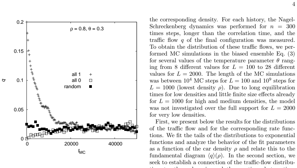
The key machinery is a biased Monte Carlo sampling of traffic histories: each history $Y$ (a sequence of $n$ Nagel-Schreckenberg updates from a fixed steady-state initial configuration) is sampled with probability $R_\theta(Y) \propto R(Y)e^{-q(Y)/\theta}$, where $\theta$ is an artificial temperature. The Metropolis–Hastings algorithm operates on the vector of random numbers that determine the history, so that $q(Y)$ becomes a deterministic function of the configuration. By combining biased histograms obtained at several $\theta$ values, the true distribution $P(q)$ is reconstructed via $P(q)=e^{q/\theta}Z(\theta)P_\theta(q)$, and the empirical rate function $\Phi(q)=-(1/L)\ln P(q)$ is computed. The exponential fits to the tails yield the slopes $m_l$ and $m_r$.
What would settle it
A direct test would be to compute the rate function for a fixed density (say $\rho=0.13$) and large system ($L=2000$) with much higher statistics and fit the left tail to an extended form such as $\ln P(q) = C + m q + k q^2$ over the same $q$ range; if $k$ is significantly nonzero, the exponential-tail assumption fails. Alternatively, an independent rare-event sampler such as importance splitting could measure $P(q)$ at a few far-tail points and be compared with the exponential extrapolation; any systematic deviation would falsify the claim.
Extended reading notes
Core claim
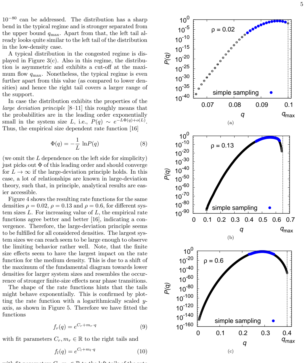
The central claim is that the rare-event properties of the Nagel-Schreckenberg model are governed by exponential tails in the flow distribution, and that the tail slopes $m_l$ and $m_r$ are characteristic functions of the car density that exhibit extrema in the vicinity of the density $\rho_{\mathrm{max}}$ at which the fundamental diagram attains its maximum. In the free-flow regime the distribution is concentrated near the maximal possible flow; near $\rho_{\mathrm{max}}$ the distribution broadens and the rate function develops a sharp bend; in the congested regime the right tail extends over a larger range. The authors interpret this as a strong relationship between the phase of the system and the shape of the large-deviation tails of the order parameter.
Load-bearing premise
The analysis treats the tails of the flow distribution as pure exponentials, so a single slope per tail fully describes the rare events; if the tails have curvature or a different functional form, the reported slope extrema and their location near $\rho_{\mathrm{max}}$ would not be a well-defined property.
Editorial extensions
If this is right
- The probability of arbitrarily large deviations in traffic flow can now be quantified: for example, events with probability as small as $10^{-13}$, which the authors argue may actually occur on a global road network within a year, become accessible to computation.
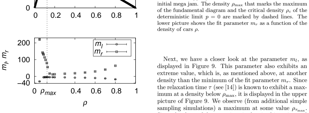
- The tail slopes $m_l$ and $m_r$ provide new density-dependent order parameters that mark the free-flow–congestion transition, possibly more sharply than the fundamental diagram itself.
- The correlation analysis shows that a given flow value is almost completely determined by the density of standing cars, even in the far tails, which may allow prediction of rare congested states from local measurements.
- The large-deviation approach can be applied to other traffic observables (jam number, jam duration) and to more realistic multi-lane or open-boundary models, as the authors state.
Reading between the lines
- The minimum of $m_r$ occurs at a density slightly above $\rho_{\mathrm{max}}$ and closer to the deterministic-limit critical density $\rho_c=1/(v_{\mathrm{max}}+1)$; the paper notes the reason is not obvious, but this hints that the right-tail statistics may be controlled by the instability of jams, not just by the steady-state flow.
- If the exponential tails are genuine, the rate function is asymptotically linear, meaning the rare events are governed by a constant 'cost' per unit flow change; this could be used to extrapolate probabilities beyond the simulated range, e.g., to estimate the risk of complete gridlock in larger systems.
- The same biasing scheme with a temperature-like parameter could be used to detect hidden phase transitions in other non-equilibrium models by monitoring the density dependence of rate-function tail slopes.
- The authors' choice to start each history from a typical steady state conditions the rare-event distribution on the typical state; an interesting extension would be to bias the initial configurations themselves to model precursors of jams, as they suggest.
Signed reviews
Editorial analysis
A structured set of objections, weighed in public.
Referee Report
Summary. The paper applies a large-deviation Monte Carlo method, with histories biased by an artificial temperature θ, to the Nagel-Schreckenberg traffic model with vmax=5 and p=0.2 on periodic lattices of size L=100–2000. It reconstructs the steady-state distribution P(q) of the traffic flow q over up to 140 orders of magnitude, defines the empirical rate function Φ(q)=-(1/L) ln P(q), observes convergence with system size, and fits exponential functions to the left and right tails of Φ. The fitted slopes ml(ρ) and mr(ρ) are reported to each have an extremum near the density ρmax where the fundamental diagram peaks; the paper also characterizes rare configurations by correlating q with the density of standing cars, the number of jams, and the average jam size, and derives simple bounds for these correlations.
Significance. If the results hold, the paper offers a useful demonstration that the large-deviation machinery can access probabilities as low as 10^-140 in a cellular-automaton traffic model, and that tail properties of the flow distribution change across the free-flow/congested crossover. The correlation analysis with the analytic bounds in Eqs. (12) and (13) provides a clear physical interpretation of rare low-flow states in terms of few large jams. The methodological strengths are the equilibration checks (Fig. 2), the overlap-based reconstruction of P(q), and the observed L-convergence of the empirical rate function (Fig. 4). However, the headline quantitative claim—the density dependence and extrema of the tail slopes—rests on the exponential ansatz in Eqs. (9)-(10), which is not made reproducible and is not tested against alternative tail shapes, and the manuscript's wording conflates the tail of P(q) with the tail of Φ(q).
major comments (3)
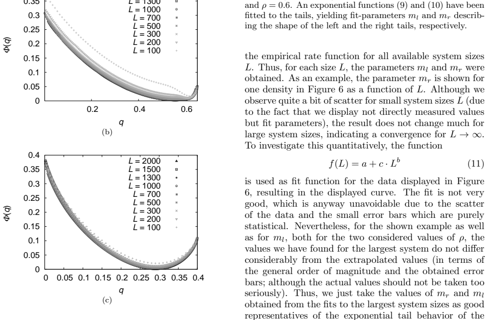
- [III A, Eqs. (9)-(10), Figs. 5 and 7] The central quantitative result, the curves ml(ρ) and mr(ρ) in Fig. 7, depends entirely on fitting the empirical rate function to exp(C+m q) over unspecified portions of the tails. The manuscript does not state the fit ranges, the number of fitted points, or the goodness of fit for any of the eighteen densities; without this information the slopes are not well defined and the reported extrema are not reproducible. Moreover, the empirical rate functions in Fig. 4 show visible curvature, so the single-exponential ansatz should be tested against alternatives such as exp(C+m q+k q^2) or a local-slope analysis. If the tails are not exponential, the fitted m is an average over an arbitrary interval, and the extrema in Fig. 7 could reflect where the fit window sits relative to the typical q rather than an intrinsic property of the model. The authors should specify all fit ranges, report how the slopes vary with the choice of window, and perform a model comparison at least for the densities displayed in Fig. 7.
- [IV (Conclusion) and Eqs. (9)-(10)] The conclusion states that the paper finds exponential left and right tails in P(q) and that the slopes of the tails change significantly. This wording is internally inconsistent with the analysis: Eqs. (9)-(10) are fitted to the rate function Φ(q), not to P(q). If Φ(q) ≈ exp(C+m q), then P(q)=exp(-L Φ(q)) ≈ exp(-L exp(C+m q)), which is not exponential in q. This is more than a stylistic issue, because it determines what physical quantity the slopes m actually characterize. The text should be rewritten so that claims are made about the rate-function tails, and any statement about P(q) itself should be derived consistently from Eq. (8).
- [III A, Fig. 6 and Eq. (11)] The extrapolation used to justify taking the largest-system fits as good representatives is not quantitatively supported. The fit f(L)=a+c L^b in Eq. (11) is described as not very good, and Fig. 6 shows substantial scatter for the smaller system sizes; the text then asserts that the largest-system values do not differ considerably from the extrapolated values without reporting the extrapolated a values or their uncertainties. This matters because the extrema of ml and mr in Fig. 7 are located by comparing slopes across nearby densities, so a systematic finite-size shift could change the apparent location. The authors should either report the extrapolated values and their uncertainties for all densities or provide a quantitative convergence criterion, for example the difference between the L=1000 and L=2000 slopes relative to the statistical error.
minor comments (4)
- [Title page and throughout] There are several typos, including 'Unversit¨at' on the title page, 'inbtroduced' in Sec. II, 'SChreckenberg' in Sec. II, and 'large-devaition' in Sec. IV; the manuscript needs a careful proofread.
- [II, Eq. (3) and following] The sign of θ needed to access the right tail is never stated explicitly. Since e^{-q/θ} suppresses large q for positive θ, the paper should say that negative values of θ are used for the right tail, or otherwise explain how the range of θ values is chosen.
- [III A and Fig. 5] The exponential-tail fits are illustrated for one density only; showing similar log-linear plots for the other densities used in Fig. 7 would allow the reader to judge whether the exponential ansatz is appropriate across the whole density range.
- [II, parameter choice] The sentence 'The general results should not depend much on the choice of these values' (referring to vmax=5 and p=0.2) is unsupported; the authors should either provide evidence or explicitly label this as a conjecture.
Circularity Check
No significant circularity: the large-deviation reconstruction is self-contained and the tail-slope analysis is an empirical fit, not a prediction derived from its inputs.
full rationale
The paper's derivation chain is not circular. The large-deviation method is fully specified in Section II: the biased distribution R_θ(Y) in Eq. (3), the exact relation Eq. (4) linking biased and unbiased distributions, the Metropolis acceptance rule Eq. (5), and the reconstruction formula Eq. (6). Although the method is attributed to Refs. [12,16,19] by the same author, the present text derives the needed equations, so the self-citations are not load-bearing; they identify prior sources rather than supply unverified content. The central empirical result — the tail slopes m_l(ρ) and m_r(ρ) of the empirical rate function Φ(q) — is obtained by fitting Eqs. (9)-(10) to measured Φ(q) data; the slopes are free fit parameters and their observed extrema near ρ_max are not forced by the definition of Φ or by the reconstruction procedure. The paper also honestly reports limitations: fit-quality caveats in Section III A ('The fit is not very good'), uncertain identification of the maximum of m_l in the Fig. 9 discussion ('we cannot decide whether the maximum of m_l coincides rather with the maximum of the relaxation time ρτmax or with the position of maximum of the fundamental diagram ρmax'), and an unexplained position of the m_r minimum in the Fig. 8 discussion ('A reason for this behavior is not obvious to us in the moment'). These are correctness/reproducibility concerns (e.g., unspecified fit intervals, untested tail shapes), not circular reductions. No equation or fitted parameter is renamed as an independent prediction, and no load-bearing step reduces by construction to its own inputs.
Assumptions & free parameters
free parameters (2)
- mr (right-tail slope of rate function) =
e.g., 29.37 +/- 0.14 for L=1000, rho=0.6
- ml (left-tail slope of rate function) =
e.g., -9.708 +/- 0.019 for L=1000, rho=0.6
assumptions (4)
- domain assumption The initial configuration y(0) is a steady-state configuration and n=300 steps is sufficient for q to be statistically independent of y(0).
- domain assumption The large-deviation principle holds for traffic flow q in the Nagel-Schreckenberg model, so the empirical rate function Phi(q) converges as L grows.
- ad hoc to paper The tails of the rate function are exponential in q, as in Eqs. (9)-(10).
- standard math The Metropolis-Hastings sampling in the biased ensemble converges to R_theta(Y) and the overlap reconstruction of P(q) is unbiased.
Cite this review
Pith. "Pith review of Rare-Event Properties of the Nagel-Schreckenberg Model." pith.science (2026). https://pith.science/paper/XVIQLUIJ
@misc{pith2026190804681,
  author       = {Pith},
  title        = {Pith review of: Rare-Event Properties of the Nagel-Schreckenberg Model},
  year         = {2026},
  howpublished = {\url{https://pith.science/paper/XVIQLUIJ}},
  note         = {Machine review of arXiv:1908.04681}
}
abstract
We have studied the distribution of traffic flow $q$ for the Nagel-Schreckenberg model by computer simulations. We applied a large-deviation approach, which allowed us to obtain the distribution $P(q)$ over more than one hundred decades in probability, down to probabilities like $10^{-140}$. This allowed us to characterize the flow distribution over a large range of the support and identify the characteristics of rare and even very rare traffic situations. We observe a change of the distribution shape when increasing the density of cars from the free flow to the congestion phase. Furthermore, we characterize typical and rare traffic situations by measuring correlations of $q$ to other quantities like density of standing cars or number and size of traffic jams.
Figures

Figures from the paper (11 more)






Reference graph
Works this paper leans on
-
[1]
Acceleration: if car i has a velocity vi <v max: vi→vi + 1
-
[2]
Slowing down due to other vehicles, preventing accidents: if the gap di =xi+1−xi− 1 between a cari and the preceding cari+1 is smaller than the velocityvi of car i: vi→di
-
[3]
Randomization: with probability p, the velocity vi of car i changes to: vi→ max (vi− 1, 0)
-
[4]
Movement: The position xi of car i is updated: xi→xi +vi For our simulations, we have chosenvmax = 5 as in the original publication, for convenience and p = 0.2. The general results should not depend much on the choice of these values. Starting with any initial configuration, simulating the Nagel-Schreckenberg dynamics is straight- forward and fast. To get...
work page 2000
-
[5]
K. Nagel and M.Schreckenberg, J. Phys. I France 2, 2221 (1992)
work page 1992
-
[6]
A. S. de Wijn, D. M. Miedema, B. Nienhuis, and 11 P. Schall, Phys. Rev. Lett. 109, 228001 (2012), URL https://link.aps.org/doi/10.1103/PhysRevLett. 109.228001
-
[7]
D. Chowdhury, L. Santen, and A. Schadschneider, Phys. Rep. 329, 100 (2000)
work page 2000
-
[8]
Helbing, Rev
D. Helbing, Rev. Mod. Phys. 73, 1067 (2001)
2001
Show all 29 references
-
[9]
Eisenbl¨ atter, L
B. Eisenbl¨ atter, L. Santen, A. Schadschneider, and M. Schreckenberg, Phys. Rev. E 57, 1309 (1998)
1998
-
[10]
Roters, S
L. Roters, S. Luebeck, and K. D. Usadel, Phys. Rev. E 59, 2672 (1999)
1999
-
[11]
Chowdhury, J
D. Chowdhury, J. Kertsz, K. Nagel, L. Santen, and A. Schadschneider, Phys. Rev. E 61, 3270 (2000)
2000
-
[12]
den Hollander, Large Deviations (American Mathe- matical Society, Providence, 2000)
F. den Hollander, Large Deviations (American Mathe- matical Society, Providence, 2000)
2000
-
[13]
Touchette, Physics Reports 478, 1 (2009), ISSN 0370- 1573
H. Touchette, Physics Reports 478, 1 (2009), ISSN 0370- 1573
2009
-
[14]
Dembo and O
A. Dembo and O. Zeitouni, Large Deviations Techniques and Applications (Springer, Berlin, 2010)
2010
-
[15]
Touchette, in Modern Computational Science 11: Lec- ture Notes from the 3rd International Oldenburg Summer School, edited by R
H. Touchette, in Modern Computational Science 11: Lec- ture Notes from the 3rd International Oldenburg Summer School, edited by R. Leidl and A. K. Hartmann (BIS- Verlag, Oldenburg, 2011), preprint arXiv:1106.4146
2011 arXiv
-
[16]
A. K. Hartmann, Phys. Rev. E 89, 052103 (2014)
2014
-
[17]
Gerwinski and J
M. Gerwinski and J. Krug, Phys. Rev. E 60, 188 (1999)
1999
-
[18]
Csanyi and J
G. Csanyi and J. Kertesz, J. Phys. A 28, L427 (1995)
1995
-
[19]
A. K. Hartmann, Big Practical guide to Computer Sim- ulation (World Scientific, 2015)
2015
-
[20]
A. K. Hartmann, Eur. Phys. J. B 84, 627 (2011)
2011
-
[21]
J. M. Hammersley and K. W. Morton, Math. Proc. Cambr. Phil. Soc. 52, 449 (1956), ISSN 1469-8064
1956
-
[22]
J. A. Bucklew, Introduction to rare event simulation (Springer-Verlag, New York, 2004)
2004
-
[23]
A. K. Hartmann, Phys. Rev. E 65, 056102 (2002)
2002
-
[24]
G. E. Crooks and D. Chandler, Phys. Rev. E 64, 026109 (2001)
2001
-
[25]
May 2019, URL https://www.cia.gov/library/publications/ the-world-factbook/geos/fr.html
CIA factbook (2019), https://www.cia.gov/library/publications/the- world-factbook/geos/fr.html, looked up 22. May 2019, URL https://www.cia.gov/library/publications/ the-world-factbook/geos/fr.html
2019
-
[26]
Engel, R
A. Engel, R. Monasson, and A. K. Hartmann, J. Stat. Phys. 117, 387 (2004)
2004
-
[27]
A. K. Hartmann, Europ. Phys. J. Spec. Topics 226, 567 (2017)
2017
-
[28]
A. K. Hartmann and M. M´ ezard, Phys. Rev. E 97, 032128 (2018)
2018
-
[29]
Schawe and A
H. Schawe and A. K. Hartmann, Eur. Phys. J. B 92, 73 (2019), URL https://doi.org/10.1140/epjb/ e2019-90667-y
2019 doi
Reviewed August 14, 2026 · model on record in the stance chip above.
Discussion (0). Continue with ORCID to comment.