Accelerating Optimization via Differentiable Stopping Time

Haoran Yuan; Yiman Fong; Zaiwen Wen; Zhonglin Xie

REVIEW 3 major objections 4 minor 37 references

Accelerating Optimization via Differentiable Stopping Time

T0 review · 3 major / 4 minor · reviewed 2026-08-07 · deepseek-v4-flash

Challenge this review Re-run · record.json Download PDF Read on arXiv ↗

Pith's one-line read The paper claims that the integer stopping time of an iterative optimization algorithm can be differentiated through an $O(h)$-accurate discrete surrogate, enabling gradient-based minimization of the iterations needed to reach a target…

desk verdict Novel surrogate for stopping-time sensitivity with a correct small-h theory, but the applications run at h=1 where the theory is silent; the idea deserves review but the empirical claims need work. read the letter →

arxiv 2505.22509 v1 pith:Y4DQSWIQ submitted 2025-05-28 cs.LG math.OC

Zhonglin Xie , Yiman Fong , Haoran Yuan , Zaiwen Wen This is my paper · ORCID

classification cs.LGmath.OC

keywords differentiablestoppingtimelearningtooptimizeonlinerateadaptationdiscreteadjointmethodcontinuous-timeoptimizationdynamicshyperparameteralgorithmacceleration

verification ladder T0 review T1 audit T2 compute T3 formal

The pith

A machine-rendered reading of the paper's core claim, the machinery that carries it, and where it could break.

The reading

The dual question of optimization—how long until the algorithm reaches a target loss?—has usually been treated as non-differentiable because the answer is an integer. The authors claim this integer stopping time can in fact be differentiated through a connection to continuous-time dynamics. They define a discrete sensitivity formula whose error relative to the true continuous stopping-time gradient is $O(h)$, and compute it with a memory-efficient discrete adjoint pass. They then use this sensitivity as a training signal in learning-to-optimize and as the basis of an online learning-rate adaptation rule for Adam, reporting fewer iterations to convergence in experiments.

What carries the argument

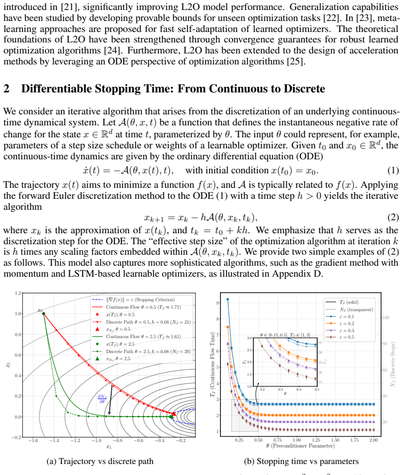
The load-bearing object is the discrete stopping-time sensitivity of Definition 3, equation (8): $\partial N/\partial\theta = -h\,\nabla J(x_N)^\top(\partial x_N/\partial\theta)/(J(x_N)-J(x_{N-1}))$. Treating the integer $N$ as a continuous variable for which $J(x_N)\approx\varepsilon$ holds, this formula formally differentiates the stopping condition; the denominator $J(x_N)-J(x_{N-1})$ approximates $h\,dJ/dt$ at the crossing, and the numerator is the state sensitivity. The discrete adjoint method (Algorithm 1) computes the vector–Jacobian products $\nabla J(x_N)^\top(\partial x_N/\partial\theta)$ and $\nabla J(x_N)^\top(\partial x_N/\partial x_0)$ by a backward recursion whose memory cost is $O(Nd+d)$, avoiding full graph unrolling. Theorem 2 is what licenses using this quantity as a stand-in for the true continuous gradient: the approximation error is first order in the step size $h$.

What would settle it

Take a simple quadratic with a preconditioner parameter $\theta$ and compute the true integer stopping time $N(\theta)$ by simulation; then compare the sign and magnitude of the surrogate gradient from (8) at $h=1$ with the finite-difference ratio $(N(\theta+\delta)-N(\theta-\delta))/(2\delta)$. If the surrogate's sign disagrees with the finite difference on a substantial fraction of $\theta$ values, the surrogate is not a descent direction and the reported acceleration could be spurious.

Watch

Extended reading notes

Core claim

The central discovery is a symbolic sensitivity for the discrete stopping time $N_J(\theta,x_0,\varepsilon)$, the first iteration at which $J(x_k)\le\varepsilon$: $\partial N/\partial\theta = -h\,\nabla J(x_N)^\top(\partial x_N/\partial\theta)/(J(x_N)-J(x_{N-1}))$, and similarly for $x_0$. Because the denominator is the one-step change in the criterion, the formula is a finite-difference surrogate for the implicit-function-theorem derivative of the continuous stopping time $T_J$, whose differentiability is established in Theorem 1. Theorem 2 bounds the gap: $\|\nabla_\theta T_J - \nabla_\theta N_J\| = O(h)$ under smoothness and a non-degenerate crossing condition. Proposition 1 shows the numerator can be obtained by a discrete adjoint recursion needing only the forward trajectory and one adjoint vector, so the sensitivity is computable without unrolling or solving an ODE. The paper then treats $\nabla_\theta N_J$ as an objective term in learning-to-optimize and derives a one-step truncated version for online learning-rate adaptation.

Load-bearing premise

The load-bearing premise is that equation (8) points in a useful descent direction for the true integer stopping time at practical step sizes such as $h=1$; the paper's $O(h)$ guarantee only holds as $h$ approaches zero.

Editorial extensions

If this is right

Learning-to-optimize objectives can be augmented with a differentiable penalty for the number of iterations to a target precision, so the learned optimizer is trained to be fast, not only to reach low loss within a fixed horizon.
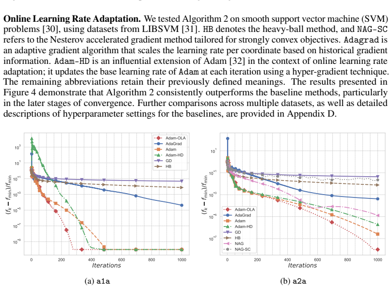
Optimizer hyperparameters such as learning rate can be adapted online from a truncated stopping-time sensitivity, yielding the Adam-OLA rule that increases the learning rate when the gradient step was beneficial and decreases it otherwise.
Because the discrete sensitivity is an $O(h)$ approximation of the continuous stopping-time gradient, algorithms that are finer discretizations of an ODE inherit a more accurate stopping-time training signal.
The discrete adjoint computation scales to high-dimensional problems (experiments go to $d=10^4$) at a fraction of the function evaluations of an adaptive ODE solver.
If the objective decreases monotonically along the trajectory, minimizing the weighted sum of losses is equivalent to greedily minimizing a sum of stopping times with weights $f(x_{k-1})-f(x_k)$ (identity (12)).

Reading between the lines

Editorial extensions of the paper, not claims the author makes directly.

The paper leaves implicit that the $O(h)$ guarantee is asymptotic; at $h=1$, the surrogate is not proven to be a descent direction for the integer stopping time, so the reported acceleration could in part be an artifact of the surrogate rather than a true decrease in the integer count.
The same finite-difference-of-criterion trick should transfer to more accurate discretizations such as symplectic or higher-order integrators, as long as the crossing condition $\nabla J^\top \dot x \neq 0$ holds; the paper mentions this as future work, but it is a natural testable extension.
One could validate the surrogate directly on small problems by comparing $\nabla_\theta N_J$ at $h=1$ against a finite difference of the integer stopping time $N_J(\theta\pm\delta)$; if signs disagree frequently, alternative surrogates would be needed.
In online adaptation, the full multi-step sensitivity back to the last adaptation point was truncated to one step; using the untruncated adjoint might give a different, possibly more stable, learning-rate schedule.

Share X Bluesky LinkedIn Reddit HN

Editorial analysis

A structured set of objections, weighed in public.

Desk editor's note, referee report, and a circularity audit.

Desk Editor's Note

read the letter

Here’s the quick take: this paper gives a clean way to define a gradient-like object for the discrete stopping time of an iterative optimizer, with a discrete adjoint to compute it cheaply. That is genuinely new as far as I can tell, and the O(h) approximation theorem is a real result. But the applications all run at h=1, where the theorem says nothing, and there is no argument that the surrogate is a descent direction for the actual integer stopping time. So the empirical speedups are suggestive, not established.

What the paper does well: Definition 3 is simple and sensible — differentiate the stopping condition J(x_N)=ε formally, treat N as continuous, and solve for ∂N/∂θ. Theorem 2 backs this up as an approximation to the continuous stopping-time gradient as h→0, with a proof that looks correct (the bound has exp factors, but that doesn't make the statement false). Algorithm 1 is a standard discrete adjoint and Proposition 1 is correct. The validation against torchdiffeq in Figure 2 is useful evidence that the discrete sensitivity actually tracks the continuous gradient at small h.

Soft spots, in order of size. First, the load-bearing gap: Theorem 2 is an asymptotic statement, and the L2O and Adam-OLA applications use h=1. The paper never addresses whether (8) is a descent direction for N_J at unit step size. The stress-test note is right that without that, the reduced iterations in Figures 3 and 4 could come from the surrogate acting as a regularizer rather than from optimizing speed-to-target. Second, equation (13) does look off by a factor of h_step relative to (8). For one step, ∂x_{k+1}/∂θ = -h_step ∂A/∂θ, so the numerator should have h_step^2 after the chain rule, unless the h in (8) is the same h_step and there's a cancelation I'm missing. The Adam application sets h_step=1, so it's unaffected, but the general formula is inconsistent. Third, the L2O experiment excludes L2O-DM because it never reaches the stopping criterion — that's a selective baseline exclusion — and there are no error bars. Fourth, Adam-OLA's hyperparameters are tuned per dataset, which weakens the comparison to baselines that use fixed search sets. The identity (12) is tautological, as the reader says; I'd not count it as a contribution.

The paper is honest in its conclusion about the limitations of Euler discretization, and the authors do not claim SOTA. I think this deserves a serious referee: the idea is new, the small-h theory is sound, and the adjoint algorithm is useful. What a referee should push on is exactly the h=1 regime and a proper empirical evaluation. If the authors can show the surrogate correlates with true stopping time at unit step sizes, or provide a counterexample where it fails, either would strengthen the paper.

Referee Report

3 major / 4 minor

Summary. The paper proposes a differentiable surrogate for the discrete stopping time of an iterative optimization algorithm. It first recalls the standard implicit-function-theorem formula for the gradient of a continuous stopping time (Theorem 1), then defines a symbolic 'sensitivity' of the integer-valued discrete stopping time in Definition 3, Eq. (8), and proves that this sensitivity approximates the continuous stopping-time gradient with O(h) error as the Euler step h tends to zero (Theorem 2). A discrete adjoint method (Algorithm 1, Proposition 1) is provided to compute the required vector-Jacobian products efficiently. The method is then applied to learning-to-optimize, with a stopping-time penalty added to the training objective, and to online learning-rate adaptation for Adam (Adam-OLA). Experiments validate the small-h approximation against an ODE solver and report reduced iteration counts in the two applications.

Significance. If the central claim held, the paper would offer a principled, gradient-based way to optimize speed-to-target rather than loss-at-a-horizon, with a memory-efficient adjoint implementation. The paper has real strengths: Theorem 1 is a standard and correct application of the implicit function theorem; Proposition 1 and Algorithm 1 correctly implement the discrete adjoint; the experiments in Section 4 confirm the O(h) approximation for small h and show computational savings relative to adaptive ODE solvers. These merits are substantial. However, the load-bearing theoretical guarantee is only asymptotic in h, while the applications run at unit step size, and the paper contains a false identity (Eq. (12)) and an inconsistent one-step formula (Eq. (13)). As a result, the paper's advertised ability to 'directly minimize the number of iterations' is not established by the evidence presented.

major comments (3)

[§2.2, Theorem 2; §3.1, §3.2] Theorem 2 guarantees only that the symbolic sensitivity (8) approximates the continuous stopping-time gradient with O(h) error as h → 0, but both applications run at h = 1: the L2O objective (10) differentiates through unit iteration steps, and Eq. (14) for Adam-OLA is Eq. (8) evaluated at h_step = 1. Moreover, the discrete stopping time N_J is integer-valued, so its true derivative is zero almost everywhere; Eq. (8) is a heuristic surrogate, not the derivative of N_J. The paper provides no theoretical or empirical argument that following this surrogate is a descent direction for N_J at h = 1. Without such an argument, the iteration-count reductions in Figures 3 and 4 could be artifacts of the surrogate acting as an arbitrary regularizer or of hyperparameter choice. A concrete fix would be to test the sign agreement between Eq. (8) and actual finite-difference changes in N_J on the experimental problems, or to include a control with a randomized or zero surrogate gradient in the L2O training.
[§3.2, Eq. (13)] Equation (13) is inconsistent with Definition 3, Eq. (8). For the single step x_{k+1} = x_k - h_step A(θ_k, x_k, t_k), we have ∂x_{k+1}/∂θ = -h_step ∂A/∂θ. Substituting this into Eq. (8) gives a numerator of h · h_step ∇J(x_{k+1})^T ∂A/∂θ, not h_step as printed in Eq. (13). The Adam-OLA derivation is numerically unaffected because h_step = 1 there, but the general one-step formula is wrong as written and should be corrected.
[§3.1, Eq. (12)] Identity (12) is not valid as stated. By Definition 2, each term N_f(θ, x_{k-1}, f(x_k)) equals exactly 1, because the next iterate generated from x_{k-1} is x_k, which satisfies f(x_k) ≤ f(x_k). Substituting N = 1 makes the right-hand side the derivative of a telescoping sum; this is not equal to Σ_k d/dθ f(x_k) whether ∂/∂θ is read as a partial derivative (the right side would be 0) or as a total derivative (the result would be b_{-1} - b_K, where b_k = ∇f(x_k)^T ∂x_k/∂θ). The claim that the sum-of-losses objective equals a sum of stopping times is therefore unsupported and should be removed or replaced with a correct statement.

minor comments (4)

[§3.1] The manuscript should state explicitly that h = 1 in the L2O experiments. Otherwise the sensitivity (8) scales with the arbitrary Euler step h even though the discrete trajectory and N_J do not, which makes the surrogate's interpretation ambiguous.
[Definition 3] The assertion that J(x_N) - J(x_{N-1}) < 0 is not a consequence of Definition 2; it is an additional monotonicity assumption on J along the iterates and should be stated as an explicit hypothesis.
[Appendix B, Eqs. (18) and (20)] The constants c1 and c2 contain the factor exp(A_x(T+1-t0)), which appears to be a typo for exp(A_x(T-t0)); please correct the exponent.
[Figure 4] The axis labels in Figure 4 appear as unicode replacement characters in the submitted file; the figure should be regenerated so that the labels are legible.

Circularity Check

1 steps flagged · score 2.0 of 10

The core O(h) approximation theorem is an independent comparison; only Eq. (12) is a definitional tautology, and the self-citation to [25] is peripheral.

self definitional [Section 3.1, Equation (12) (L2O with Differentiable Stopping Time)]
"Suppose f (xk) > f(xk+1) holds for all k, another interesting result comes from the identity d dθ KmaxX k=0 f (xk) = KmaxX k=0 (f (xk) − f (xk−1)) ∇f (xk)∂xk/∂θ f (xk) − f (xk−1) = ∂ ∂θ KmaxX k=0 (f (xk−1) − f (xk))Nf (θ, xk−1, f(xk)). (12) The identity (12) reveals that optimizing the weighted loss sum with wk ≡ 1 equals to minimize the sum of stopping times greedily with stopping criterion f and natural weights f (xk−1) − f (xk)."

With Definition 2, Nf(θ, xk−1, f(xk)) is the first index n≥0 with f(xn)≤f(xk) when the trajectory starts at xk−1. The paper assumes f(xk)>f(xk+1) for all k, so f(xk−1)>f(xk) and the very next iterate xk already satisfies the threshold: Nf(...)=1 by construction. Inserting Nf=1 makes the right side of (12) a derivative of Σ(f(xk−1)−f(xk)), i.e. a rearrangement of the chain-rule terms on the left. The advertised equivalence between the loss sum and a greedy sum of stopping times is therefore not an independent derivation but a definitional tautology. This identity is a side remark in Section 3.1 and is not used to prove Theorem 2 or to generate the empirical speedups.

full rationale

The central derivation is not circular. Theorem 1 derives the continuous stopping-time gradient by the implicit function theorem. Definition 3 introduces a new symbolic discrete sensitivity (8). Theorem 2 then proves, via standard forward-Euler error estimates (Proposition 2 and the bounds in Appendix B), that this discrete object approaches the independently defined continuous gradient as h→0. The proof does not assume its conclusion, and the two objects are not identified by construction. Proposition 1 is a direct adjoint chain-rule computation, and the numerical validation compares against an independent torchdiffeq solver. The self-citation to [25] is peripheral: it supports a path-differentiability remark and a comment on future improvements of the h→0 estimate, so it is not load-bearing. The serious gap that Theorem 2 is asymptotic in h while the L2O and Adam-OLA applications run at h=1 is a soundness or validation issue, not circularity; the paper itself flags the fixed-step limitation in the Conclusion. The only circular-adjacent step is Eq. (12): by Definition 2, Nf(θ, xk−1, f(xk))=1 because the next iterate already meets the threshold, so the claimed identity reduces to a rearrangement of chain-rule terms. This is a side remark and is not used to prove Theorem 2 or to produce the reported speedups, so the overall circularity score is low.

Assumptions & free parameters 4 free parameters · 4 assumptions · 0 invented entities

The theoretical results rest on standard ODE and implicit-function theorems plus regularity assumptions. The empirical claims rest on several hand-set hyperparameters and a heuristic surrogate gradient that is not proven to be a valid descent direction at the step sizes used.

free parameters (4)

eta_adapt (Adam-OLA adaptation rate) = 1e-2 to 5e-5 per dataset (Table 1)
Controls the magnitude of the learning-rate update in Algorithm 2; selected per dataset.
epsilon (descent threshold in Adam-OLA) = 1e-5 to 5e-9 per dataset (Table 1)
Triggers when to apply the learning-rate adaptation; tuned per dataset.
lambda (stopping-time penalty weight in L2O) = 1 in experiments, 0 baseline
Balances the dense loss and the stopping-time penalty in equation (10); chosen by hand.
L2O stopping criterion epsilon = f(x_{k-1}) - f(x_k) <= 1e-5
Defines the discrete stopping time for the penalty; selected without theoretical justification.

assumptions (4)

domain assumption The iterative algorithm (2) is exactly the forward Euler discretization of an underlying ODE (1).
All theory and applications rely on this modeling assumption (Section 2).
domain assumption The stopping criterion J and dynamics A are smooth with bounded derivatives up to second order, and the boundary condition ∇J(x(T_J))^T ẋ(T_J) ≠ 0 holds.
Needed for Theorems 1 and 2; guarantees the sensitivity formula does not degenerate.
domain assumption The discrete stopping index N_J satisfies T_J ∈ (t_{N_J-1}, t_{N_J}], i.e., the continuous crossing occurs between the last two discrete iterates.
Assumed in Theorem 2; fails if discretization error moves the crossing to a different interval.
ad hoc to paper The surrogate sensitivity (8) is an acceptable substitute for the gradient of the integer stopping time even at h=1.
Applications use unit step size; no proof of descent direction at this step size.

how reviews work

0 comments

Cite this review

Pith. "Pith review of Accelerating Optimization via Differentiable Stopping Time." pith.science (2026). https://pith.science/paper/Y4DQSWIQ

@misc{pith2026250522509,
  author       = {Pith},
  title        = {Pith review of: Accelerating Optimization via Differentiable Stopping Time},
  year         = {2026},
  howpublished = {\url{https://pith.science/paper/Y4DQSWIQ}},
  note         = {Machine review of arXiv:2505.22509}
}

read the original abstract

Optimization is an important module of modern machine learning applications. Tremendous efforts have been made to accelerate optimization algorithms. A common formulation is achieving a lower loss at a given time. This enables a differentiable framework with respect to the algorithm hyperparameters. In contrast, its dual, minimizing the time to reach a target loss, is believed to be non-differentiable, as the time is not differentiable. As a result, it usually serves as a conceptual framework or is optimized using zeroth-order methods. To address this limitation, we propose a differentiable stopping time and theoretically justify it based on differential equations. An efficient algorithm is designed to backpropagate through it. As a result, the proposed differentiable stopping time enables a new differentiable formulation for accelerating algorithms. We further discuss its applications, such as online hyperparameter tuning and learning to optimize. Our proposed methods show superior performance in comprehensive experiments across various problems, which confirms their effectiveness.

Figures

Figures reproduced from arXiv: 2505.22509 by the authors.

**Figure 2.** Experimental results comparing the discrete and continuous stopping time gradients across [PITH_FULL_IMAGE:figures/full_fig_p008_2.png] view at source ↗

**Figure 3.** Test results of different optimizers on logistic regression: Function value versus iteration. [PITH_FULL_IMAGE:figures/full_fig_p009_3.png] view at source ↗

Figures from the paper (3 more)

**Figure 4.** Figure 4: Comparison of different optimizers on smooth SVM: Function value versus iteration. Here, [PITH_FULL_IMAGE:figures/full_fig_p009_4.png]

**Figure 5.** Figure 5: NFEs of different solvers. Hyperparameters of Baselines. Adagrad is an adaptive gradient algorithm that adjusts learning rates per coordinate based on historical gradient information. The learning rate is set β ∈ {10−3 , 10−2 , 10−1 , 1.0, 10.0, 1/L} with ϵ = 10−8 . F…

**Figure 6.** Figure 6: Comparison of different optimizers on smooth SVM: Function value versus iteration. Here, [PITH_FULL_IMAGE:figures/full_fig_p019_6.png]

Discussion (0). Continue with ORCID to comment.

Reference graph

Works this paper leans on

37 extracted references · 34 canonical work pages

[1]

Operations research: an introduction, volume 7

Hamdy A Taha and Hamdy A Taha. Operations research: an introduction, volume 7. Prentice hall Upper Saddle River, NJ, 1997

work page 1997
[2]

A survey of large language models, 2025

Wayne Xin Zhao, Kun Zhou, Junyi Li, Tianyi Tang, Xiaolei Wang, Yupeng Hou, Yingqian Min, Beichen Zhang, Junjie Zhang, Zican Dong, Yifan Du, Chen Yang, Yushuo Chen, Zhipeng Chen, Jinhao Jiang, Ruiyang Ren, Yifan Li, Xinyu Tang, Zikang Liu, Peiyu Liu, Jian-Yun Nie, and Ji-Rong Wen. A survey of large language models, 2025. URL https://arxiv.org/abs/ 2303.18223

arXiv 2025
[3]

Finance and financial markets

Keith Pilbeam. Finance and financial markets. Bloomsbury Publishing, 2018

work page 2018
[4]

Hyperparameter optimization

Matthias Feurer and Frank Hutter. Hyperparameter optimization. Springer International Publishing, 2019

work page 2019
[5]

Learning to optimize: A tutorial for continuous and mixed-integer optimization

Xiaohan Chen, Jialin Liu, and Wotao Yin. Learning to optimize: A tutorial for continuous and mixed-integer optimization. Science China Mathematics, 67(6):1191–1262, 2024

work page 2024
[6]

Problem complexity and method efficiency in optimization

Arkadij Semenoviˇc Nemirovskij and David Borisovich Yudin. Problem complexity and method efficiency in optimization. Wiley-Interscience, 1983

work page 1983
[7]

A differential equation for modeling nesterov’s accelerated gradient method: Theory and insights

Weijie Su, Stephen Boyd, and Emmanuel J Candes. A differential equation for modeling nesterov’s accelerated gradient method: Theory and insights. Journal of Machine Learning Research, 17(1):5312–5354, 2016

work page 2016
[8]

Understanding the acceleration phenomenon via high-resolution differential equations

Bin Shi, Simon S Du, Michael I Jordan, and Weijie J Su. Understanding the acceleration phenomenon via high-resolution differential equations. Mathematical Programming, 194: 313–351, 2022

work page 2022

Show all 37 references

[9]

Acceleration via symplectic discretiza- tion of high-resolution differential equations

Bin Shi, Simon S Du, Weijie Su, and Michael I Jordan. Acceleration via symplectic discretiza- tion of high-resolution differential equations. In Advances in Neural Information Processing Systems, pages 5745–5753, 2019

2019
[10]

A lyapunov analysis for accelerated gradient methods: From deterministic to stochastic case

Mathieu Laborde and Adam Oberman. A lyapunov analysis for accelerated gradient methods: From deterministic to stochastic case. In International Conference on Artificial Intelligence and Statistics, pages 602–612. PMLR, 2020

2020
[11]

Accelerated natural gradient method for parametric manifold optimization, 2025

Chenyi Li, Shuchen Zhu, Zhonglin Xie, and Zaiwen Wen. Accelerated natural gradient method for parametric manifold optimization, 2025. URL https://arxiv.org/abs/2504.05753

2025 arXiv
[12]

Efficient and modular implicit differentiation

Mathieu Blondel, Quentin Berthet, Marco Cuturi, Roy Frostig, Stephan Hoyer, Felipe Llinares- López, Fabian Pedregosa, and Jean-Philippe Vert. Efficient and modular implicit differentiation. In Advances in Neural Information Processing Systems, volume 35, pages 14502–14514, 2022

2022
[13]

Nonsmooth implicit differen- tiation for machine-learning and optimization

Jérôme Bolte, Tam Le, Edouard Pauwels, and Jean-Philippe Vert. Nonsmooth implicit differen- tiation for machine-learning and optimization. In Advances in Neural Information Processing Systems, volume 34, pages 11913–11924, 2021

2021
[14]

Object representations as fixed points: Training iterative refinement algorithms with implicit differentiation

Michael Chang, Thomas Griffiths, and Sergey Levine. Object representations as fixed points: Training iterative refinement algorithms with implicit differentiation. In Advances in Neural Information Processing Systems, volume 35, pages 22838–22849, 2022. 10

2022
[15]

Implicit differentiation for fast hyperparameter selection in non-smooth convex learning

Quentin Bertrand, Quentin Klopfenstein, Mathieu Massias, Mathieu Blondel, Gael Varoquaux, Alexandre Gramfort, and Joseph Salmon. Implicit differentiation for fast hyperparameter selection in non-smooth convex learning. Journal of Machine Learning Research , 23(1): 7710–7749, 2022

2022
[16]

On training implicit models

Zhengyang Geng, Xin-Yu Zhang, Shaoyuan Bai, Yiran Wang, and Zhouchen Lin. On training implicit models. In Advances in Neural Information Processing Systems, volume 34, pages 3562–3575, 2021

2021
[17]

On implicit bias in overparameterized bilevel optimization

Paul Vicol, Jonathan P Lorraine, Fabian Pedregosa, Juan-Manuel Pérez-Rua, and Pierre Ablin. On implicit bias in overparameterized bilevel optimization. In International Conference on Machine Learning, pages 22137–22161. PMLR, 2022

2022
[18]

Revisiting implicit differentiation for learning problems in optimal control

Ming Xu, Timothy L Molloy, and Stephen Gould. Revisiting implicit differentiation for learning problems in optimal control. In Advances in Neural Information Processing Systems, volume 36, pages 66428–66441, 2023

2023
[19]

Learning to optimize: A primer and a benchmark

Tianlong Chen, Xiaohan Chen, Wuyang Chen, Howard Heaton, Jialin Liu, Zhangyang Wang, and Wotao Yin. Learning to optimize: A primer and a benchmark. Journal of Machine Learning Research, 23:1–20, 2022

2022
[20]

Scalable learning to optimize: A learned optimizer can train big models

Xinyang Chen, Tianlong Chen, Yinghua Cheng, Wuyang Chen, Xiaoyang Xiao, Ziyi Lu, and Zhangyang Wang. Scalable learning to optimize: A learned optimizer can train big models. In European Conference on Computer Vision, pages 377–394. Springer, 2022

2022
[21]

Training stronger baselines for learning to optimize

Tianlong Chen, Weiyi Zhang, Zhou Jingyang, Shiyu Wang, Wei Zhang, and Zhangyang Wang. Training stronger baselines for learning to optimize. In Advances in Neural Information Processing Systems, volume 33, pages 10658–10669, 2020

2020
[22]

Learning to generalize provably in learning to optimize

Jiayi Yang, Tianlong Chen, Muxin Zhu, Fengxiang He, Dacheng Tao, and Zhangyang Wang. Learning to generalize provably in learning to optimize. InInternational Conference on Machine Learning, pages 39496–39519. PMLR, 2023

2023
[23]

M-l2o: Towards generalizable learning-to-optimize by test-time fast self-adaptation

Jiayi Yang, Xinyang Chen, Tianlong Chen, Zhangyang Wang, and Yingbin Liang. M-l2o: Towards generalizable learning-to-optimize by test-time fast self-adaptation. arXiv preprint arXiv:2303.00039, 2023

2023 arXiv
[24]

Towards robust learning to optimize with theoretical guarantees

Qi Song, Weiyang Lin, Jingyi Wang, and Hao Xu. Towards robust learning to optimize with theoretical guarantees. In Proceedings of the IEEE Conference on Computer Vision and Pattern Recognition, 2024

2024
[25]

ODE-based Learning to Optimize, 2024

Zhonglin Xie, Wotao Yin, and Zaiwen Wen. ODE-based Learning to Optimize, 2024. URL https://arxiv.org/abs/2406.02006

2024 arXiv
[26]

Conservative set valued fields, automatic differentiation, stochastic gradient methods and deep learning

Jérôme Bolte and Edouard Pauwels. Conservative set valued fields, automatic differentiation, stochastic gradient methods and deep learning. Mathematical Programming, 188:19–51, 2021

2021
[27]

Ricky T. Q. Chen, Yulia Rubanova, Jesse Bettencourt, and David Duvenaud. Neural ordinary differential equations. In Advances in Neural Information Processing Systems, volume 31, 2018

2018
[28]

Hoffman, David Pfau, Tom Schaul, and Nando de Freitas

Marcin Andrychowicz, Misha Denil, Sergio Gomez Colmenarejo, Matthew W. Hoffman, David Pfau, Tom Schaul, and Nando de Freitas. Learning to learn by gradient descent by gradient descent. In Daniel D. Lee, Masashi Sugiyama, Ulrike von Luxburg, Isabelle Guyon, and Roman Garnett, e...

2016
[29]

Learning gradient descent: Better generalization and longer horizons

Kaifeng Lv, Shunhua Jiang, and Jian Li. Learning gradient descent: Better generalization and longer horizons. In Doina Precup and Yee Whye Teh, editors, Proceedings of the 34th International Conference on Machine Learning, ICML 2017, Sydney, NSW, Australia, 6-11 August 2017, v...

2017
[30]

Yuh-Jye Lee and O. L. Mangasarian. SSVM: A smooth support vector machine for classification. Comput. Optim. Appl. , 20(1):5–22, 2001. doi: 10.1023/A:1011215321374. URL https: //doi.org/10.1023/A:1011215321374

2001 doi
[31]

LIBSVM: A library for support vector machines

Chih-Chung Chang and Chih-Jen Lin. LIBSVM: A library for support vector machines. ACM Transactions on Intelligent Systems and Technology, 2:27:1–27:27, 2011. Software available at http://www.csie.ntu.edu.tw/~cjlin/libsvm

2011
[32]

Online learning rate adaptation with hypergradient descent

Atilim Gunes Baydin, Robert Cornish, David Martínez-Rubio, Mark Schmidt, and Frank Wood. Online learning rate adaptation with hypergradient descent. In 6th International Conference on Learning Representations, ICLR 2018, Vancouver, BC, Canada, April 30 - May 3, 2018, Conferenc...

2018
[33]

Provable and practical online learning rate adaptation with hypergradient descent, 2025

Ya-Chi Chu, Wenzhi Gao, Yinyu Ye, and Madeleine Udell. Provable and practical online learning rate adaptation with hypergradient descent, 2025. URL https://arxiv.org/abs/ 2502.11229

2025 arXiv
[34]

Towards constituting mathematical structures for learning to optimize

Jialin Liu, Xiaohan Chen, Zhangyang Wang, Wotao Yin, and HanQin Cai. Towards constituting mathematical structures for learning to optimize. In Proceedings of the 40th International Conference on Machine Learning, pages 21426–21449, 2023. 12 A Proof of Theorem 1 Proof. Consider...

2023
[35]

There exists a constant Lx > 0 such that ∥f (x1, t) − f (x2, t)∥ ≤Lx∥x1 − x2∥ for all x1, x2, and t
[36]

There exists a constant Lt > 0 such that ∥f (x, t1) − f (x, t2)∥ ≤Lt|t1 − t2| for all x, t1, and t2
[37]

Given an initial condition x(t0) = x0 and a fixed stepsize h, we consider the sequence generated by the forward Euler method as xk+1 = xk + hf (xk, tk), t k = t0 + kh

There exists a constant M >0 such that ∥f (x, t)∥ < Mfor all x and t. Given an initial condition x(t0) = x0 and a fixed stepsize h, we consider the sequence generated by the forward Euler method as xk+1 = xk + hf (xk, tk), t k = t0 + kh. Then, for any positive integer k, the e...

Pith tools

Reviewed August 7, 2026 · model on record in the stance chip above.

[1] [1]

Operations research: an introduction, volume 7

Hamdy A Taha and Hamdy A Taha. Operations research: an introduction, volume 7. Prentice hall Upper Saddle River, NJ, 1997

work page 1997

[2] [2]

A survey of large language models, 2025

Wayne Xin Zhao, Kun Zhou, Junyi Li, Tianyi Tang, Xiaolei Wang, Yupeng Hou, Yingqian Min, Beichen Zhang, Junjie Zhang, Zican Dong, Yifan Du, Chen Yang, Yushuo Chen, Zhipeng Chen, Jinhao Jiang, Ruiyang Ren, Yifan Li, Xinyu Tang, Zikang Liu, Peiyu Liu, Jian-Yun Nie, and Ji-Rong Wen. A survey of large language models, 2025. URL https://arxiv.org/abs/ 2303.18223

arXiv 2025

[3] [3]

Finance and financial markets

Keith Pilbeam. Finance and financial markets. Bloomsbury Publishing, 2018

work page 2018

[4] [4]

Hyperparameter optimization

Matthias Feurer and Frank Hutter. Hyperparameter optimization. Springer International Publishing, 2019

work page 2019

[5] [5]

Learning to optimize: A tutorial for continuous and mixed-integer optimization

Xiaohan Chen, Jialin Liu, and Wotao Yin. Learning to optimize: A tutorial for continuous and mixed-integer optimization. Science China Mathematics, 67(6):1191–1262, 2024

work page 2024

[6] [6]

Problem complexity and method efficiency in optimization

Arkadij Semenoviˇc Nemirovskij and David Borisovich Yudin. Problem complexity and method efficiency in optimization. Wiley-Interscience, 1983

work page 1983

[7] [7]

A differential equation for modeling nesterov’s accelerated gradient method: Theory and insights

Weijie Su, Stephen Boyd, and Emmanuel J Candes. A differential equation for modeling nesterov’s accelerated gradient method: Theory and insights. Journal of Machine Learning Research, 17(1):5312–5354, 2016

work page 2016

[8] [8]

Understanding the acceleration phenomenon via high-resolution differential equations

Bin Shi, Simon S Du, Michael I Jordan, and Weijie J Su. Understanding the acceleration phenomenon via high-resolution differential equations. Mathematical Programming, 194: 313–351, 2022

work page 2022