REVIEW 3 major objections 6 minor 40 references
ST-VTD, a tensor decomposition with low-rank spatial and LSTM temporal priors, recovers latent fMRI-like factors with spatial and temporal correlations near 0.98, outperforming classical and probabilistic decomposition baselines.
Reviewed by Pith at T0; open to challenge. T0 means a machine referee read the full paper against a public rubric. the ladder, T0–T4 →
T0 review · deepseek-v4-flash
2026-08-01 05:18 UTC pith:YFBBQ4YU
load-bearing objection A genuinely new synthesis of LL1-style spatial priors, LSTM temporal priors, and LPALM amortized variational inference, but the central empirical claim is undercut by the GICA warm-start confound and the synthetic-only evaluation. the 3 major comments →
Variational Low-rank Tensor Decomposition for Multisubject Spatiotemporal Data Analysis
The pith
A machine-rendered reading of the paper's core claim, the machinery that carries it, and where it could break.
Core claim
The central claim is that subject-specific spatial maps and temporal dynamics in multisubject spatiotemporal data can be jointly modeled as latent factors with structured priors — low-rank spatial maps inspired by LL1 and LSTM-driven temporal courses — and inferred with an amortized variational posterior built by unrolling LPALM iterations. If this is right, ST-VTD recovers the underlying components more accurately than GICA, LL1, Bayesian CP factorization, and PARAFAC2 on the synthetic benchmark: corr_z=0.9829, corr_c=0.9845, re_z=0.1578, re_c=0.1605, against best-baseline correlations around 0.93 and errors above 0.25. The ablation supports the design: dropping the LSTM prior or the low-ra
What carries the argument
The central mechanism is a bilinear generative model X^{(n)} = sum_k Z_k^{(n)} ∘ c_k^{(n)} + Gaussian noise, combined with two structured priors: each spatial map is centered at a low-rank product U_k V_k^T with a shared per-component variance (LL1-inspired), and each temporal course is centered at the output of a learned LSTM with per-component variance. The posterior is made tractable by a conditional mean-field variational approximation whose means are computed by unrolling I=50 iterations of LPALM, the linearized proximal alternating least-squares update, with a hard low-rank SVD projection on the spatial columns; small MLPs output the log-variances. The GICA warm start provides the init
Load-bearing premise
The load-bearing premise is that the synthetic evaluation is a valid substitute for real multisubject fMRI: the benchmark data are generated from the same bilinear low-rank plus Gaussian-noise model ST-VTD assumes, so violations such as motion artifacts, scanner effects, heavy-tailed noise, or missing data could erase the reported gains.
What would settle it
Generate a multisubject spatiotemporal benchmark from realistic fMRI-like spatial templates with heavy-tailed noise, motion-related outliers, and a percentage of missing time points, then fit ST-VTD and the four baselines; if ST-VTD no longer achieves the highest correlations and lowest factor errors, the paper's central claim about latent recovery on its own benchmark would not generalize.
If this is right
- If correct, ST-VTD recovers latent fMRI-like components with correlations around 0.98 on synthetic multisubject data, substantially above the tested baselines.
- The framework supports swapping priors, update rules, and projection constraints within the same variational formulation, so it can be adapted without redesigning inference.
- The ablations indicate the LSTM temporal prior, the low-rank spatial prior, and the hard low-rank projection each contribute to the reported gains.
- The GICA-based warm start is important for the non-convex optimization; random initialization leads to a large degradation in component recovery.
- Because the posterior means are used as MMSE estimates, the model naturally produces uncertainty intervals alongside point estimates for each spatial and temporal factor.
Where Pith is reading between the lines
- Editorial inference: the modularity of the design suggests a direct stress test the paper does not run — keep the LPALM-unrolled posterior exactly as is, replace the LSTM temporal prior with a simpler linear Gaussian prior, and measure how much temporal recovery drops; this would isolate how much of the gain comes from the temporal prior versus the unrolled inference.
- Editorial inference: since GICA initialization is nearly load-bearing, a spectral or multi-start initialization selected by the ELBO could make the method applicable where group ICA models are invalid (e.g., data with nonstationary mixing), a route the paper leaves open.
- Editorial inference: if the reported correlations transfer to real fMRI, the per-component variational variances could be used as statistical confidence maps for spatial-network discovery, a clinical use case the paper does not evaluate.
Editorial analysis
A structured set of objections, weighed in public.
Referee Report
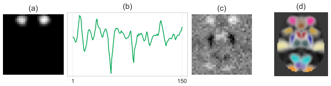
Summary. The paper introduces ST-VTD, a variational framework for multisubject spatiotemporal tensor data that combines a bilinear outer-product generative model (Eq. (1)) with a low-rank spatial prior inspired by LL1 and an LSTM-based temporal prior. Posterior inference is amortized and implemented by unrolling LPALM iterations, with a GICA-based warm start. Experiments on a synthetic fMRI-like dataset (N=100, T=150, 30×30 spatial resolution, K=10 components) compare ST-VTD with GICA, LL1, BCPF, and PARAFAC2. The central claim is that ST-VTD achieves the best latent-factor recovery, with corr_z=0.9829, corr_c=0.9845, re_z=0.1578, re_c=0.1605, while also matching the best reconstruction error. The paper includes an ablation study of modeling choices and a random-initialization check, and the code is publicly available.
Significance. If the central claim holds, ST-VTD offers a useful contribution to multisubject fMRI-style tensor decomposition: it combines structured spatial and temporal priors with a parameter-efficient amortized variational inference scheme and demonstrates strong latent recovery on a synthetic benchmark. The paper's strengths include a reproducible experimental setup, public code, a clear ablation of the proposed priors and projection scheme, and a transparent discussion of the GICA-warm-start dependence. However, the empirical claim currently rests on a controlled synthetic dataset generated from the same bilinear outer-product model family assumed by ST-VTD, and the comparison is complicated by an asymmetric initialization: ST-VTD is initialized from GICA solutions while baselines are run standalone. The missing warm-start control and the absence of statistical significance testing are load-bearing for the claim that the proposed variational framework, rather than fine-tuning of a privileged initialization, is responsible for the reported gains.
major comments (3)
- [§III-C, §III-D, Table I] The warm-start asymmetry is not controlled. ST-VTD is initialized from GICA outputs (Z(0)=Z_GICA+Δz, C(0)=C_GICA+Δc) and then trained for 150 Adam epochs, while GICA and the other baselines are run standalone. The ablation in §III-C shows that random initialization degrades re_z and re_c by ≈335% and correlations by ≈30%, implying that without the GICA warm start ST-VTD would be worse than GICA (re_z≈0.68 vs 0.525 in Table I). To support the claim that the variational framework, the LSTM prior, and the low-rank spatial prior provide the benefit, the authors should add a control that refines the GICA solution with the same unrolled LPALM updates and Adam training but without the variational KL terms and LSTM prior. Without this control, the Table I ordering may be attributable to additional fine-tuning of a strong initialization rather than to the proposed model.
- [§III-A, §IV] The evaluation is conducted under model match. Section IV states that the benchmark is 'a controlled synthetic dataset generated according to the proposed generative model,' i.e., the same bilinear outer-product structure as Eq. (1) with subject-specific factors, Gaussian noise, and smooth spatial/temporal components. Since the ground truth is generated from exactly the model family that ST-VTD assumes, the reported advantage over baselines may not transfer to real fMRI data containing non-Gaussian artifacts, missing observations, scanner effects, or structures outside the low-rank + LSTM prior family. The authors should add model-mismatch experiments (e.g., non-Gaussian noise, missing entries, different generating mechanisms) or an application to real data before claiming that ST-VTD 'significantly improves latent factor recovery' in a general sense. The acknowledgment in the conclusion
- [§III-D, Table I] No statistical significance testing is reported. Table I lists means and standard deviations, but the central claim is based on point estimates. For example, the reconstruction error difference between ST-VTD and LL1 is 0.2524 vs 0.2527, well within the reported standard deviations, and several baseline correlation metrics have large variability (e.g., LL1 corr_z = 87.4±24.9). The authors should provide paired tests across repeated synthetic instantiations or across subjects, and report effect sizes or confidence intervals. Without this, the statement that ST-VTD 'outperforms all baselines' is not statistically supported, especially where the differences are small relative to variance.
minor comments (6)
- [§II-A, Eq. (3)] The notation New(·,·) is defined, but it would help to state explicitly that p(Z_k) in Eq. (3) is a matrix-variate Gaussian written entrywise; the low-rank mean Uk V_k^T plus λ_k^2 I is a valid prior, but the identifiability of U_k and V_k under the likelihood is not discussed. A brief note on this would improve clarity.
- [§II-B] The unrolled LPALM updates use a matrix representation X∈R^{T×V}, Z∈R^{V×K}, C∈R^{T×K}; however, the generative model in Eq. (1) defines X^{(n)} as a third-order tensor. The reshaping from tensor to matrix is implicit and should be stated explicitly, especially because the low-rank projection P_LR reshapes columns of Z back into Vx×Vy matrices.
- [§III-C] The description of the learnable offset Δz, Δc says it is 'shared across subjects,' but the later text refers to 'subject-shared learnable offset.' This is consistent, but the phrase 'small subject-shared' could confuse; suggest rewording to 'shared across all subjects.'
- [§III-D, Fig. 2] The caption says the subject is 'n=1 across models' and that ST-VTD achieved the median reconstruction error, but it is unclear whether n=1 is the same subject for all methods or whether each method's median subject is displayed. Please clarify.
- [Table I] The table caption states 'All values are multiplied by 100.' For readability, consider using percentages or fractions consistently, and note whether the standard deviations are over subjects or over independent synthetic trials.
- [§II-A] The LSTM prior in Eq. (4) sets p(c_k)=New(w(t,θ_k), γ_k). The input t is a vector of time coordinates, but the mechanism by which the LSTM produces a deterministic mean vector of length T is not specified; a sentence on the LSTM architecture (input, hidden state, output layer) would help reproducibility.
Circularity Check
No significant circularity: the paper's empirical benchmark is model-matched but not definitionally equivalent, and the GICA warm-start is a confound, not a circular reduction.
full rationale
I found no step in which a claimed prediction reduces, by the paper's own equations or by a self-citation chain, to its input. The generative model in Eq. (1) is used as the likelihood for ST-VTD and also as the template for the synthetic benchmark, but the recovery of latent factors from noisy data is still a nontrivial inference problem, and all baselines are evaluated on the same data. Section IV's statement that the evaluation used 'a controlled synthetic dataset generated according to the proposed generative model' is an explicitly acknowledged limitation on external validity, not a circular construction: the ground-truth factors are not fed into the estimator, and the reported correlations/errors are measured against known targets. The GICA warm-start described in Section III-C is a legitimate concern for attribution — the ablation shows random initialization degrades recovery by roughly 335% and correlations drop by about 30% — but this is an experimental confound (missing a control where GICA is refined with the same unrolled updates without the variational terms), not a definitional equivalence. No equation in the paper makes the final ST-VTD estimate equal to the GICA input, nor is any benchmark metric forced by construction. Self-citations in the references are background citations for existing tensor-decomposition and fMRI methods; they do not carry the load of the paper's central empirical claim. Therefore the paper is not circular.
Axiom & Free-Parameter Ledger
free parameters (7)
- Spatial low-rank rank L = floor(min(Vx,Vy)/K) =
3 (for Vx=Vy=30, K=10)
- Number of components K =
10
- Spatial prior factors U_k, V_k and variances lambda_k^2 =
learned during training (not reported)
- LSTM temporal prior weights theta_k and variances gamma_k =
learned during training (not reported)
- Likelihood noise variance sigma^2 =
not reported; presumably optimized as part of theta
- KL annealing coefficients beta_max_z, beta_max_c and warm-up steps W_z, W_c =
5, 5, 50, 50
- Variational encoder parameters (MLP variance heads, unrolled LPALM offsets) =
learned (~19,300 total trainable parameters)
axioms (6)
- domain assumption Each subject tensor equals a sum of K outer products of spatial and temporal factors plus i.i.d. Gaussian noise (Eq. 1).
- domain assumption Spatial maps live near a rank-L manifold with L = floor(min(Vx,Vy)/K) (Eq. 3 and projection P_LR).
- domain assumption Temporal courses can be represented by a shared-parameter LSTM with Gaussian residual (Eq. 4).
- domain assumption The Neuromark-based synthetic data with perturbations and Gaussian noise is a realistic proxy for real fMRI.
- domain assumption Mean-field conditional Gaussian variational family is sufficiently expressive for the posterior.
- domain assumption Truncated SVD column-wise projection is the correct low-rank structure for spatial maps.
read the original abstract
Modeling shared and subject-specific structure in multisubject spatiotemporal data remains challenging, particularly in neuroimaging, where both spatial and temporal patterns exhibit rich variability across subjects. Existing matrix and tensor decompositions provide interpretable factorizations, but rely on fixed multilinear structures or coupling schemes that may limit their flexibility in capturing complex variability. In this work, we introduce a spatiotemporal variational tensor decomposition (ST-VTD) framework that combines a tensor factorization generative model with structured priors to jointly represent spatial maps and temporal dynamics. Spatial factors are regularized to promote a low-rank structure inspired by the LL1 decomposition, while temporal factors are modeled using a learned Long short-term memory (LSTM)-based prior, enabling flexible and adaptive dynamics. Posterior inference is performed using an amortized variational formulation by unrolling iterations of an optimization algorithm, leading to an interpretable and parameter-efficient architecture. The proposed inference framework employs a warm-start strategy based on group independent component analysis, which we found to improve optimization performance. Experiments on a realistic synthetic functional MRI (fMRI) dataset demonstrate that the proposed approach significantly improves latent factor recovery compared with representative classical and probabilistic decomposition benchmarks.
Figures

Reference graph
Works this paper leans on
-
[1]
Empirical orthogonal functions and related techniques in atmospheric science: A review,
A. Hannachi, I. T. Jolliffe, and D. B. Stephenson, “Empirical orthogonal functions and related techniques in atmospheric science: A review,” International Journal of Climatology, vol. 27, no. 9, pp. 1119–1152, 2007
2007
-
[2]
Blind fMRI source unmixing via higher-order tensor decompositions,
C. Chatzichristos, E. Kofidis, M. Morante, and S. Theodoridis, “Blind fMRI source unmixing via higher-order tensor decompositions,”Journal of Neuroscience Methods, vol. 315, pp. 17–47, 2019
2019
-
[3]
A review of change detection in multitemporal hyperspectral images: Current techniques, applications, and challenges,
S. Liu, D. Marinelli, L. Bruzzone, and F. Bovolo, “A review of change detection in multitemporal hyperspectral images: Current techniques, applications, and challenges,”IEEE Geoscience and Remote Sensing Magazine, vol. 7, no. 2, pp. 140–158, 2019
2019
-
[4]
Reproducibility in Matrix and Tensor Decompositions: Focus on model match, interpretability, and uniqueness,
T. Adali, F. Kantar, M. A. B. S. Akhonda, S. Strother, V . D. Calhoun, and E. Acar, “Reproducibility in Matrix and Tensor Decompositions: Focus on model match, interpretability, and uniqueness,”IEEE Signal Processing Magazine, vol. 39, no. 4, pp. 8–24, 2022
2022
-
[5]
Personalized coupled tensor decomposition for multimodal data fusion: Uniqueness and algo- rithms,
R. A. Borsoi, K. Usevich, D. Brie, and T. Adali, “Personalized coupled tensor decomposition for multimodal data fusion: Uniqueness and algo- rithms,”IEEE Transactions on Signal Processing, vol. 73, pp. 113–129, 2024
2024
-
[6]
Multimodal Data Fusion: An Overview of Methods, Challenges, and Prospects,
D. Lahat, T. Adali, and C. Jutten, “Multimodal Data Fusion: An Overview of Methods, Challenges, and Prospects,”Proceedings of the IEEE, vol. 103, no. 9, pp. 1449–1477, 2015
2015
-
[7]
Data fusion in metabolomics using coupled matrix and tensor factorizations,
E. Acar, R. Bro, and A. K. Smilde, “Data fusion in metabolomics using coupled matrix and tensor factorizations,”Proceedings of the IEEE, vol. 103, no. 9, pp. 1602–1620, 2015
2015
-
[8]
Coupled tensor decomposition for hyperspectral and multispectral image fusion with inter-image variability,
R. A. Borsoi, C. Pr ´evost, K. Usevich, D. Brie, J. C. Bermudez, and C. Richard, “Coupled tensor decomposition for hyperspectral and multispectral image fusion with inter-image variability,”IEEE Journal of Selected Topics in Signal Processing, vol. 15, no. 3, pp. 702–717, 2021
2021
-
[9]
Coupled tensor decompositions for data fusion,
C. Chatzichristos, S. Van Eyndhoven, E. Kofidis, and S. Van Huffel, “Coupled tensor decompositions for data fusion,” inTensors for data processing. Elsevier, 2022, pp. 341–370
2022
-
[10]
A review of group ICA for fMRI data and ICA for joint inference of imaging, genetic, and erp data,
V . D. Calhoun, J. Liu, and T. Adalı, “A review of group ICA for fMRI data and ICA for joint inference of imaging, genetic, and erp data,” Neuroimage, vol. 45, no. 1, pp. S163–S172, 2009
2009
-
[11]
Tensor decompositions and applications,
T. G. Kolda and B. W. Bader, “Tensor decompositions and applications,” SIAM Review, vol. 51, no. 3, pp. 455–500, 2009
2009
-
[12]
Tensor decomposition for signal processing and machine learning,
N. D. Sidiropoulos, L. De Lathauwer, X. Fu, K. Huang, E. E. Papalex- akis, and C. Faloutsos, “Tensor decomposition for signal processing and machine learning,”IEEE Transactions on signal processing, vol. 65, no. 13, pp. 3551–3582, 2017
2017
-
[13]
Coupled canonical polyadic decompositions and (coupled) decompositions in multilinear rank- (Lr,n, Lr,n,1)terms–part I: Uniqueness,
M. Sørensen and L. D. De Lathauwer, “Coupled canonical polyadic decompositions and (coupled) decompositions in multilinear rank- (Lr,n, Lr,n,1)terms–part I: Uniqueness,”SIAM Journal on Matrix Analysis and Applications, vol. 36, no. 2, pp. 496–522, 2015
2015
-
[14]
Learning spatiotemporal brain dynamics in adolescents via multimodal MEG and fMRI data fusion using joint tensor/matrix decomposition,
I. Belyaeva, B. Gabrielson, Y .-P. Wang, T. W. Wilson, V . D. Calhoun, J. M. Stephen, and T. Adali, “Learning spatiotemporal brain dynamics in adolescents via multimodal MEG and fMRI data fusion using joint tensor/matrix decomposition,”IEEE Transactions on Biomedical Engineering, vol. 71, no. 7, pp. 2189–2200, 2024
2024
-
[15]
An AO-ADMM approach to constraining PARAFAC2 on all modes,
M. Roald, C. Schenker, V . D. Calhoun, T. Adali, R. Bro, J. E. Cohen, and E. Acar, “An AO-ADMM approach to constraining PARAFAC2 on all modes,”SIAM Journal on Mathematics of Data Science, vol. 4, no. 3, pp. 1191–1222, 2022
2022
-
[16]
Coupled CP tensor decomposition with shared and distinct components for multi-task fMRI data fusion,
R. A. Borsoi, I. Lehmann, M. A. B. S. Akhonda, V . D. Calhoun, K. Usevich, D. Brie, and T. Adali, “Coupled CP tensor decomposition with shared and distinct components for multi-task fMRI data fusion,” in Proc. IEEE International Conference on Acoustics, Speech and Signal Processing (ICASSP), vol. 51, 2023, pp. 1–5
2023
-
[17]
Exploring multimodal data fusion through joint decompositions with flexible couplings,
R. C. Farias, J. E. Cohen, and P. Comon, “Exploring multimodal data fusion through joint decompositions with flexible couplings,”IEEE Transactions on Signal Processing, vol. 64, no. 18, pp. 4830–4844, 2016
2016
-
[18]
Bayesian CP factorization of incomplete tensors with automatic rank determination,
Q. Zhao, L. Zhang, and A. Cichocki, “Bayesian CP factorization of incomplete tensors with automatic rank determination,”IEEE Transac- tions on Pattern Analysis and Machine Intelligence, vol. 37, no. 9, pp. 1751–1763, 2015
2015
-
[19]
Diversity in Independent Com- ponent and Vector Analyses: Identifiability, algorithms, and applications in medical imaging,
T. Adali, M. Anderson, and G.-S. Fu, “Diversity in Independent Com- ponent and Vector Analyses: Identifiability, algorithms, and applications in medical imaging,”IEEE Signal Processing Magazine, vol. 31, no. 3, pp. 18–33, 2014
2014
-
[20]
Neural topographic factor analysis for fMRI data,
E. Sennesh, Z. Khan, Y . Wang, J. B. Hutchinson, A. Satpute, J. Dy, and J.-W. van de Meent, “Neural topographic factor analysis for fMRI data,”Advances in Neural Information Processing Systems, vol. 33, pp. 12 046–12 056, 2020
2020
-
[21]
Deep markov factor analysis: Towards concurrent temporal and spatial analysis of fMRI data,
A. Farnoosh and S. Ostadabbas, “Deep markov factor analysis: Towards concurrent temporal and spatial analysis of fMRI data,”Advances in Neural Information Processing Systems, vol. 34, pp. 17 876–17 888, 2021
2021
-
[22]
Undirected probabilistic model for tensor decomposition,
Z. Tao, T. Tanaka, and Q. Zhao, “Undirected probabilistic model for tensor decomposition,”Advances in Neural Information Processing Systems, vol. 36, pp. 25 837–25 853, 2023
2023
-
[23]
Unrolling PALM for sparse semi-blind source separation,
M. Fahes, C. Kervazo, J. Bobin, and F. Tupin, “Unrolling PALM for sparse semi-blind source separation,” inInternational Conference on Learning Representations, 2022
2022
-
[24]
Tensors: a brief introduction,
P. Comon, “Tensors: a brief introduction,”IEEE Signal Processing Magazine, vol. 31, no. 3, pp. 44–53, 2014
2014
-
[25]
Decompositions of a higher-order tensor in block terms—part II: Definitions and uniqueness,
L. De Lathauwer, “Decompositions of a higher-order tensor in block terms—part II: Definitions and uniqueness,”SIAM Journal on Matrix Analysis and Applications, vol. 30, no. 3, pp. 1033–1066, 2008
2008
-
[26]
On uniqueness and computation of the decomposition of a tensor into multilinear rank-(1, L r, Lr)terms,
I. Domanov and L. D. Lathauwer, “On uniqueness and computation of the decomposition of a tensor into multilinear rank-(1, L r, Lr)terms,” SIAM Journal on Matrix Analysis and Applications, vol. 41, no. 2, pp. 747–803, 2020
2020
-
[27]
Hyperspectral super-resolution accounting for spectral variability: Coupled tensor LL1-based recovery and blind unmixing of the unknown super-resolution image,
C. Pr ´evost, R. A. Borsoi, K. Usevich, D. Brie, J. C. Bermudez, and C. Richard, “Hyperspectral super-resolution accounting for spectral variability: Coupled tensor LL1-based recovery and blind unmixing of the unknown super-resolution image,”SIAM Journal on Imaging Sciences, vol. 15, no. 1, pp. 110–138, 2022
2022
-
[28]
Fast and structured block-term tensor decomposition for hyperspectral unmixing,
M. Ding, X. Fu, and X.-L. Zhao, “Fast and structured block-term tensor decomposition for hyperspectral unmixing,”IEEE Journal of Selected Topics in Applied Earth Observations and Remote Sensing, vol. 16, pp. 1691–1709, 2023
2023
-
[29]
H. Sak, A. Senior, and F. Beaufays, “Long short-term memory based recurrent neural network architectures for large vocabulary speech recognition,” 2014. [Online]. Available: https://arxiv.org/abs/1402.1128
Pith/arXiv arXiv 2014
-
[30]
C. M. Bishop,Pattern Recognition and Machine Learning. Springer, 2006
2006
-
[31]
Deep unrolling of the multiplicative updates algorithm for blind source separation, with appli- cation to hyperspectral unmixing,
C. Kervazo, A. Chetoui, and J. E. Cohen, “Deep unrolling of the multiplicative updates algorithm for blind source separation, with appli- cation to hyperspectral unmixing,” in32nd European Signal Processing Conference (EUSIPCO). EURASIP, 2024, pp. 656–660
2024
-
[32]
Algorithm unrolling: Interpretable, efficient deep learning for signal and image processing,
V . Monga, Y . Li, and Y . C. Eldar, “Algorithm unrolling: Interpretable, efficient deep learning for signal and image processing,”IEEE Signal Processing Magazine, vol. 38, no. 2, pp. 18–44, 2021
2021
-
[33]
K. P. Murphy,Machine learning: A probabilistic perspective. MIT press, 2012
2012
-
[34]
An introduction to variational autoen- coders,
P. K. Diederik and W. Max, “An introduction to variational autoen- coders,”F oundations and Trends® in Machine Learning, vol. 12, no. 4, pp. 307–392, 2019
2019
-
[35]
Auto-encoding variational bayes,
D. P. Kingma and M. Welling, “Auto-encoding variational bayes,” in International Conference on Learning Representations, 2014
2014
-
[36]
beta-V AE: Learning basic visual concepts with a constrained variational framework,
I. Higgins, L. Matthey, A. Pal, C. P. Burgess, X. Glorot, M. M. Botvinick, S. Mohamed, and A. Lerchner, “beta-V AE: Learning basic visual concepts with a constrained variational framework,” inInterna- tional Conference on Learning Representations, 2016
2016
-
[37]
Cyclical annealing schedule: A simple approach to mitigating KL vanishing,
H. Fu, C. Li, X. Liu, J. Gao, A. Celikyilmaz, and L. Carin, “Cyclical annealing schedule: A simple approach to mitigating KL vanishing,” in Proc. NAACL-HLT 2019, V olume 1 (Long and Short Papers), 2019, pp. 240–250
2019
-
[38]
Neuromark: An automated and adaptive ICA based pipeline to identify reproducible fMRI markers of brain disorders,
Y . Du, Z. Fu, J. Sui, S. Gao, Y . Xing, D. Lin, M. Salman, A. Abrol, M. A. Rahaman, J. Chenet al., “Neuromark: An automated and adaptive ICA based pipeline to identify reproducible fMRI markers of brain disorders,” NeuroImage: Clinical, vol. 28, p. 102375, 2020
2020
-
[39]
Independent component analysis: algorithms and applications,
A. Hyv ¨arinen and E. Oja, “Independent component analysis: algorithms and applications,”Neural networks, vol. 13, no. 4-5, pp. 411–430, 2000
2000
-
[40]
Vervliet, O
N. Vervliet, O. Debals, L. Sorber, M. Van Barel, and L. De Lathauwer. (2016) Tensorlab 3.0. [Online]. Available: https://www.tensorlab.net
2016
discussion (0)
Sign in with ORCID, Apple, or X to comment. Anyone can read and Pith papers without signing in.