REVIEW 4 major objections 6 minor 31 references
Backpropagation-Free Metropolis-Adjusted Langevin Algorithm
T0 review · 4 major / 6 minor · reviewed 2026-08-07 · deepseek-v4-flash
Pith's one-line read The paper introduces the first backpropagation-free gradient-based MCMC algorithm, folding random tangent directions from forward-mode automatic differentiation into MALA proposals and reporting competitive or better sampling on several…
desk verdict New and useful idea with a real memory advantage, but the best sampler's pseudocode is internally inconsistent and the missing stationarity proof is a serious gap. read the letter →
The pith
A machine-rendered reading of the paper's core claim, the machinery that carries it, and where it could break.
The reading
What carries the argument
The load-bearing mechanism is the random unit tangent vector $\hat v \sim \mathrm{Uniform}(S^{D-1})$, which serves simultaneously as the direction for the forward-mode Jacobian-vector product and as an auxiliary variable in the proposal. Because the uniform density is constant, $q(\hat v^*)=q(\hat v_t)$ cancels in the Metropolis-Hastings acceptance ratio, which the paper uses to keep the target at $p(\theta)$. Forward-mode evaluation returns $f(\theta)$, $\nabla f(\theta)\cdot \hat v$, and in the second-order case $\hat v^\top \nabla^2 f(\theta)\hat v$ in one pass; the absolute value of that quadratic form gives a position-specific curvature scale for preconditioning. The line variants reduce the proposal to a one-dimensional Gaussian along the sampled direction, which the experiments show makes step-size tuning less delicate.
What would settle it
Run the line samplers on a high-dimensional isotropic Gaussian target and compare the empirical marginal variances to the known posterior: if the chains mix but the recovered variances are systematically biased, or if the acceptance ratio fails a detailed-balance check for some step size, the central claim that forward-only gradients preserve the MALA target is falsified.
Extended reading notes
Core claim
Central to the paper is the observation that the tangent vector already required by forward-mode automatic differentiation can be treated as an auxiliary variable in a Metropolis-Hastings step. Sampling $\hat v$ uniformly from the unit sphere $S^{D-1}$ makes its density constant, so the tangent probabilities cancel from the acceptance ratio; the remaining update uses only the directional derivative $\nabla f(\theta)\cdot \hat v$ and, for the second-order variants, the quadratic form $\hat v^\top \nabla^2 f(\theta)\hat v$. From this the paper constructs four samplers: Forward MALA, Line Forward MALA, Preconditioned Forward MALA, and Preconditioned Line Forward MALA. The reported experiments show forward-mode samplers matching or beating reverse-mode MALA on multinomial logistic regression and Bayesian neural network regression, and avoiding the out-of-memory failure that MALA hits on a 2.4-million-parameter CNN.
Load-bearing premise
The construction assumes that adding a uniformly random tangent direction as an auxiliary variable, and cancelling its density in the acceptance ratio, leaves $p(\theta)$ as the stationary distribution; the paper does not prove detailed balance or ergodicity for this augmented chain.
Editorial extensions
If this is right
- Because no backward pass or stored activations are needed, the forward-mode samplers can run within memory budgets where reverse-mode MALA fails; the paper reports MALA running out of memory on a 2.4-million-parameter CNN while forward-mode variants continue.
- Average time per MCMC step falls by roughly 25 to 34 percent in the reported logistic-regression and CNN experiments, with accuracy and calibration comparable to MALA.
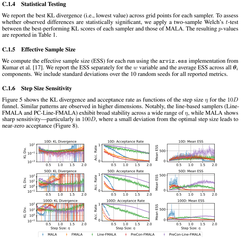
- The line-based variants, Line-FMALA and PC-Line-FMALA, are less sensitive to step-size choice than MALA, which simplifies tuning in practice.
- PC-Line-FMALA, which combines the line constraint with second-order preconditioning, is often the best forward-mode sampler across the funnel, logistic-regression, and BNN-regression experiments.
Reading between the lines
- Not in the paper: the same tangent-vector cancellation could be dropped into Hamiltonian Monte Carlo or stochastic-gradient MCMC, potentially producing a broader family of backprop-free samplers beyond MALA.
- Not in the paper: because the unit-sphere gradient estimator's variance grows with dimension, the reported high-dimensional successes likely come from the line-based and preconditioned variants; a variance-per-unit-cost comparison across samplers would make this explicit.
- Not in the paper: antithetic or stratified tangent directions might reduce forward-gradient variance without backpropagation, an extension that could strengthen the line samplers and is directly testable with the code released for the paper.
Editorial analysis
A structured set of objections, weighed in public.
Referee Report
Summary. The paper proposes four forward-mode automatic-differentiation variants of the Metropolis-Adjusted Langevin Algorithm (FMALA, Line-FMALA, PC-FMALA, and PC-Line-FMALA). The central idea is to sample a tangent vector as an auxiliary variable so that proposals use only Jacobian-vector products (and, for the preconditioned variants, Hessian-vector products), eliminating the backward pass required by reverse-mode MALA. The authors claim to be the first to introduce backpropagation-free gradient-based MCMC, report results on a funnel distribution, MNIST logistic regression, a Bayesian neural network regression, and a CIFAR-10 CNN, and argue that the forward-mode samplers are competitive with MALA while offering lower memory and sometimes lower runtime.
Significance. If the samplers are correct and the experiments are reproducible, this is a useful contribution to gradient-based MCMC, especially for memory-constrained Bayesian deep learning. The idea of using the sampled tangent direction as an auxiliary variable with a uniform-sphere density that cancels in the acceptance ratio is elegant, and the line-sampler variants are a natural extension. The variance analysis of the normalized-tangent gradient estimator in Section 4.4 and Appendix B is a solid auxiliary result. However, the manuscript does not supply a stationarity proof for the proposed kernels, Algorithm 4 contains an internal inconsistency in its reverse proposal, and the main empirical claims are weakened by best-of-grid selection before p-value computation and by asymmetric tuning in the BNN experiments. The central claims are plausible but not yet fully supported.
major comments (4)
- [§4.2 / Algorithm 2 and §4.3.2 / Algorithm 4] The paper does not prove that Line-FMALA and PC-Line-FMALA have p(θ) as their stationary distribution. Because the line samplers propose moves on a one-dimensional affine subspace and sample a fresh tangent direction each iteration, correctness requires an explicit detailed-balance argument on the augmented distribution p(θ)U(v) — for example, treating the sampler as a Gibbs step on v followed by a Metropolis step restricted to the sampled line. As written, the acceptance ratio in Algorithm 2 uses the same v in the forward and reverse Gaussian densities, which is valid only if v is part of the persistent state; the manuscript does not say this. Please provide a formal correctness proof or a precise statement of the augmented-state construction.
- [Appendix A, Algorithm 4] Algorithm 4 is internally inconsistent in the reverse proposal. The step labeled "Evaluate components of q(αt|α∗, v)" calls F2(θ∗, v∗) with a freshly sampled v∗, but the mean µPLFM(α∗, v, η) and the variance in the acceptance ratio use the original v. If an implementation follows the F2(θ∗, v∗) call, the reverse proposal is not the reverse of the forward move along the original line, and detailed balance can fail; if the implementation correctly uses v throughout, the F2(θ∗, v∗) evaluation is a typographical error. Since PC-Line-FMALA is the best-performing algorithm in Tables 1, 2, and 3, this must be resolved by correcting the pseudocode and by stating explicitly which evaluation the released code uses.
- [Table 1 and Appendix C.1.4] The p-values reported against MALA are computed on the single grid point that minimizes KL for each sampler. Selecting the best of 100 step sizes before applying a two-sample Welch t-test invalidates the p-value interpretation, because the selected best-order statistic is biased and no multiple-comparison correction is applied. Please report the full grid comparison as in Figure 8 with a corrected testing protocol, or use a pre-specified step size for each sampler.
- [Table 3 and Appendix C.3.2] The BNN regression results (Table 3) report NLL and MSE without error bars or repeated-seed variability, and Appendix C.3.2 states that for MALA the step size was further fine-tuned and the burn-in was separately optimized, while forward-mode samplers used a fixed 10^4 burn-in. This asymmetric tuning budget, combined with the missing uncertainty estimates, does not support the claim that the line-based forward samplers outperform MALA in NLL. Please report repeated-seed results with error bars and ensure all samplers receive the same tuning and burn-in optimization protocol.
minor comments (6)
- [Appendix B, variance derivation] In the sentence discussing moment identities, the phrase "cross terms E[ˆv^2_i] = 0" should instead state that E[ˆv_i ˆv_j] = 0 for i ≠ j; the second-moment notation is otherwise clear.
- [§4.4] The sentence "asymptotically recovers the same variance as D → ∞" should specify that it refers to the variance of the scaled estimator D·ĝ_i, not to the raw estimator ĝ_i; the current wording is ambiguous.
- [Tables 2 and 3] Tables 2 and 3 report NLL, accuracy, and ECE without error bars; please indicate whether these are single runs or averages over multiple seeds and, if averaged, report standard deviations.
- [§5.4 / Figure 7] The CNN experiment reports only the best step-size results in Table 4; please state explicitly how the grid was selected and whether the same grid procedure was used for all samplers, and consider reporting the full grid as is done for the funnel distribution.
- [Notation throughout] The abbreviations for the preconditioned line sampler are inconsistent: PC-Line-FMALA in Algorithm 4, PC-L-FMALA in Tables 1 and 5, and PreCon-Line-FMALA in the text. Please unify the notation.
- [§2 Related work] The novelty claim "first to introduce backpropagation-free gradient-based MCMC" should be tempered or contextualized with a discussion of existing line-sampling and random-direction MCMC methods (e.g., hit-and-run) and of stochastic-gradient MCMC, since those are conceptually adjacent and are not currently cited.
Circularity Check
No circularity: the samplers are defined from explicit proposal mechanisms and evaluated on external benchmarks, with no fitted quantity renamed as a prediction.
full rationale
The paper's derivation chain is self-contained in the relevant sense. Each of the four samplers is defined by an explicit proposal equation (Eqs. 5, 6, 8, 9), and the Metropolis-Hastings acceptance ratios in Algorithms 1-4 are written directly in terms of the target log-density and the Gaussian proposal densities, with the uniform tangent-vector densities cancelling because they are equal by construction. No parameter is fitted to the reported performance metrics and then presented as a prediction; the step-size selection in the experiments is standard hyperparameter tuning, and the Appendix B variance analysis is a direct calculation using standard moments of the uniform distribution on the sphere, not an assumption of the paper's own conclusions. The bias correction in App. B.1 multiplies tangent vectors by sqrt(D) and re-derives the proposal forms; it is an algebraic rescaling rather than a result imported from the paper's own claims. Prior work cited (Baydin et al. for forward gradients, Girolami and Calderhead for preconditioned MALA) is external background and is not used to justify the paper's central novelty or performance claims. The apparent inconsistency in Algorithm 4, where a fresh v* is sampled for the reverse proposal in the pseudocode while the acceptance ratio uses v, is a correctness and reversibility concern rather than a circularity concern, because the claimed stationary distribution is not being assumed as an input anywhere in the construction. Therefore no load-bearing step reduces to its own inputs by definition, by fitting, or by self-citation.
Assumptions & free parameters
free parameters (1)
- Step size eta per sampler and model =
Tuned by grid search or Bayesian optimization; exact values not reported
assumptions (4)
- domain assumption Metropolis-Hastings acceptance with auxiliary tangent vector v preserves the target distribution p(theta)
- standard math For v uniformly distributed on the unit sphere, E[v_i^2]=1/D and E[v_i^4]=3/[D(D+2)]
- domain assumption Forward-mode AD costs roughly twice a single function evaluation and does not store intermediate activations
- standard math The Euler-discretized Langevin proposal followed by MH correction is a valid MCMC construction
Cite this review
Pith. "Pith review of Backpropagation-Free Metropolis-Adjusted Langevin Algorithm." pith.science (2026). https://pith.science/paper/YGUKGRQ4
@misc{pith2026250518081,
  author       = {Pith},
  title        = {Pith review of: Backpropagation-Free Metropolis-Adjusted Langevin Algorithm},
  year         = {2026},
  howpublished = {\url{https://pith.science/paper/YGUKGRQ4}},
  note         = {Machine review of arXiv:2505.18081}
}
read the original abstract
Recent work on backpropagation-free learning has shown that it is possible to use forward-mode automatic differentiation (AD) to perform optimization on differentiable models. Forward-mode AD requires sampling a tangent vector for each forward pass of a model. The result is the model evaluation with the directional derivative along the tangent. In this paper, we illustrate how the sampling of this tangent vector can be incorporated into the proposal mechanism for the Metropolis-Adjusted Langevin Algorithm (MALA). As such, we are the first to introduce a backpropagation-free gradient-based Markov chain Monte Carlo (MCMC) algorithm. We also extend to a novel backpropagation-free position-specific preconditioned forward-mode MALA that leverages Hessian information. Overall, we propose four new algorithms: Forward MALA; Line Forward MALA; Pre-conditioned Forward MALA, and Pre-conditioned Line Forward MALA. We highlight the reduced computational cost of the forward-mode samplers and show that forward-mode is competitive with the original MALA, while even outperforming it depending on the probabilistic model. We include Bayesian inference results on a range of probabilistic models, including hierarchical distributions and Bayesian neural networks.
Figures


Figures from the paper (3 more)


Reference graph
Works this paper leans on
-
[1]
Methods of information geometry, volume 191
Shun-ichi Amari and Hiroshi Nagaoka. Methods of information geometry, volume 191. Ameri- can Mathematical Soc., 2000
work page 2000
-
[2]
Gradients without backpropagation
Atılım Güne¸ s Baydin, Barak A Pearlmutter, Don Syme, Frank Wood, and Philip Torr. Gradients without backpropagation. arXiv preprint arXiv:2202.08587, 2022
arXiv 2022
-
[3]
Towards biologically plausible deep learning
Yoshua Bengio, Dong-Hyun Lee, Jorg Bornschein, Thomas Mesnard, and Zhouhan Lin. Towards biologically plausible deep learning. arXiv preprint arXiv:1502.04156, 2015
arXiv 2015
-
[4]
A general metric for Riemannian manifold Hamiltonian Monte Carlo
Michael Betancourt. A general metric for Riemannian manifold Hamiltonian Monte Carlo. In International Conference on Geometric Science of Information, pages 327–334. Springer, 2013
work page 2013
-
[5]
JAX: composable transformations of Python+NumPy programs, 2018
James Bradbury, Roy Frostig, Peter Hawkins, Matthew James Johnson, Chris Leary, Dougal Maclaurin, George Necula, Adam Paszke, Jake VanderPlas, Skye Wanderman-Milne, and Qiao Zhang. JAX: composable transformations of Python+NumPy programs, 2018. URL https://github.com/google/jax
work page 2018
-
[6]
Second-order forward-mode automatic differentiation for optimization
Adam D Cobb, Atılım Güne¸ s Baydin, Barak A Pearlmutter, and Susmit Jha. Second-order forward-mode automatic differentiation for optimization. arXiv preprint arXiv:2408.10419, 2024
arXiv 2024
-
[7]
Simon Duane, Anthony D Kennedy, Brian J Pendleton, and Duncan Roweth. Hybrid Monte Carlo. Physics letters B, 195(2):216–222, 1987
work page 1987
-
[8]
Can forward gradient match backpropagation? In International Conference on Machine Learning, pages 10249–10264
Louis Fournier, Stéphane Rivaud, Eugene Belilovsky, Michael Eickenberg, and Edouard Oyallon. Can forward gradient match backpropagation? In International Conference on Machine Learning, pages 10249–10264. PMLR, 2023
2023
Show all 31 references
-
[9]
Riemann manifold Langevin and Hamiltonian Monte Carlo methods
Mark Girolami and Ben Calderhead. Riemann manifold Langevin and Hamiltonian Monte Carlo methods. Journal of the Royal Statistical Society Series B: Statistical Methodology, 73 (2):123–214, 2011
2011
-
[10]
Evaluating derivatives: principles and techniques of algorithmic differentiation
Andreas Griewank and Andrea Walther. Evaluating derivatives: principles and techniques of algorithmic differentiation. SIAM, 2008
2008
-
[11]
The forward-forward algorithm: Some preliminary investigations
Geoffrey Hinton. The forward-forward algorithm: Some preliminary investigations. arXiv preprint arXiv:2212.13345, 2022
2022 arXiv
-
[12]
The No-U-Turn sampler: adaptively setting path lengths in Hamiltonian Monte Carlo
Matthew D Hoffman, Andrew Gelman, et al. The No-U-Turn sampler: adaptively setting path lengths in Hamiltonian Monte Carlo. J. Mach. Learn. Res., 15(1):1593–1623, 2014
2014
-
[13]
Subspace inference for Bayesian deep learning
Pavel Izmailov, Wesley J Maddox, Polina Kirichenko, Timur Garipov, Dmitry Vetrov, and Andrew Gordon Wilson. Subspace inference for Bayesian deep learning. In Uncertainty in Artificial Intelligence, pages 1169–1179. PMLR, 2020
2020
-
[14]
What are Bayesian neural network posteriors really like? In International conference on machine learning, pages 4629–4640
Pavel Izmailov, Sharad Vikram, Matthew D Hoffman, and Andrew Gordon Gordon Wilson. What are Bayesian neural network posteriors really like? In International conference on machine learning, pages 4629–4640. PMLR, 2021
2021
-
[15]
Decoupled neural interfaces using synthetic gradients
Max Jaderberg, Wojciech Marian Czarnecki, Simon Osindero, Oriol Vinyals, Alex Graves, David Silver, and Koray Kavukcuoglu. Decoupled neural interfaces using synthetic gradients. In International conference on machine learning, pages 1627–1635. PMLR, 2017. 10
2017
-
[16]
Learning multiple layers of features from tiny images
Alex Krizhevsky, Geoffrey Hinton, et al. Learning multiple layers of features from tiny images. 2009
2009
-
[17]
ArviZ a unified library for exploratory analysis of Bayesian models in Python
Ravin Kumar, Colin Carroll, Ari Hartikainen, and Osvaldo Martin. ArviZ a unified library for exploratory analysis of Bayesian models in Python. Journal of Open Source Software, 4(33): 1143, 2019. doi: 10.21105/joss.01143. URL https://doi.org/10.21105/joss.01143
2019 doi
-
[18]
Gradient-based learning applied to document recognition
Yann LeCun, Léon Bottou, Yoshua Bengio, and Patrick Haffner. Gradient-based learning applied to document recognition. Proceedings of the IEEE, 86(11):2278–2324, 1998
1998
-
[19]
Bayesian Learning for Neural Networks
Radford M Neal. Bayesian Learning for Neural Networks. PhD thesis, University of Toronto, 1995
1995
-
[20]
Slice sampling
Radford M Neal. Slice sampling. The annals of statistics, 31(3):705–767, 2003
2003
-
[21]
MCMC Using Hamiltonian Dynamics
Radford M Neal. MCMC Using Hamiltonian Dynamics. In Handbook of Markov Chain Monte Carlo, pages 113–162. Chapman and Hall/CRC, 2011
2011
-
[22]
Pytorch: An imperative style, high-performance deep learning library
Adam Paszke, Sam Gross, Francisco Massa, Adam Lerer, James Bradbury, Gregory Chanan, Trevor Killeen, Zeming Lin, Natalia Gimelshein, Luca Antiga, et al. Pytorch: An imperative style, high-performance deep learning library. Advances in neural information processing systems, 32, 2019
2019
-
[23]
Fast exact multiplication by the Hessian
Barak A Pearlmutter. Fast exact multiplication by the Hessian. Neural Computation, 6(1): 147–160, 1994
1994
-
[24]
Scaling forward gradient with local losses
Mengye Ren, Simon Kornblith, Renjie Liao, and Geoffrey Hinton. Scaling forward gradient with local losses. arXiv preprint arXiv:2210.03310, 2022
2022 arXiv
-
[25]
Langevin diffusions and metropolis-hastings algorithms
Gareth O Roberts and Osnat Stramer. Langevin diffusions and metropolis-hastings algorithms. Methodology and computing in applied probability, 4:337–357, 2002
2002
-
[26]
Rosenbrock
H. Rosenbrock. An automatic method for finding the greatest or least value of a function. The Computer Journal, 3(3):175–184, 1960
1960
-
[27]
Brownian dynamics as smart Monte Carlo simulation
Peter J Rossky, Jimmie D Doll, and Harold L Friedman. Brownian dynamics as smart Monte Carlo simulation. The Journal of Chemical Physics, 69(10):4628–4633, 1978
1978
-
[28]
Learning by directional gradient descent
David Silver, Anirudh Goyal, Ivo Danihelka, Matteo Hessel, and Hado van Hasselt. Learning by directional gradient descent. In International Conference on Learning Representations, 2021
2021
-
[29]
A simple automatic derivative evaluation program
Robert Edwin Wengert. A simple automatic derivative evaluation program. Communications of the ACM, 7(8):463–464, 1964
1964
-
[30]
Langevin diffusions and the Metropolis-adjusted Langevin algorithm
Tatiana Xifara, Chris Sherlock, Samuel Livingstone, Simon Byrne, and Mark Girolami. Langevin diffusions and the Metropolis-adjusted Langevin algorithm. Statistics & Proba- bility Letters, 91:14–19, 2014. 11 A Algorithms Algorithm 1 Forward-Mode Metropolis Adjusted Langevin Dyn...
2014
-
[31]
/homes/usr/lib/scripts/Sampling/cifar10_cnn/cifar10_time.py
+ X j̸=i ∂f ∂θj 2 1 D(D + 2) + 2 X j̸=i X k̸=i,k>j ∂f ∂θj ∂f ∂θk [0] = 1 D(D + 2) 3 ∂f ∂θi 2 + X j̸=i ∂f ∂θj 2 . Finally, the variance is given by Var (ˆgi(θ)) = 1 D(D + 2) 2 (D − 1) D ∂f ∂θi 2 + X j̸=i ∂f ∂θj 2 . If we multiply the original estimator by D to mak...
Reviewed August 7, 2026 · model on record in the stance chip above.
Discussion (0). Sign in to comment.