REVIEW 3 major objections 5 minor 54 references
Returning Back to Mukhanov Parametrization of Inflationary Equation of State
T0 review · 3 major / 5 minor · reviewed 2026-08-11 · deepseek-v4-flash
Pith's one-line read The Mukhanov inflation parametrization is viable only for 1.5 < α ≤ 2.2.
desk verdict The Mukhanov parametrization paper has a fatal internal inconsistency: the end-of-inflation condition forces β = 2/3, so the two-parameter treatment and all derived constraints are not well-posed. read the letter →
The pith
A machine-rendered reading of the paper's core claim, the machinery that carries it, and where it could break.
The reading
What carries the argument
The machinery is the Hamilton-Jacobi formalism, in which the Hubble parameter $H$ is the fundamental quantity rather than the inflaton potential. Its central identity is $\epsilon_H=2M_P^2(H'/H)^2=\frac{3}{2}(1+\omega)$, so the Mukhanov parametrization becomes $\epsilon_H=\frac{3\beta}{2(N+1)^\alpha}$. Integrating $dN=\epsilon_H^{-1}\,dH/H$ gives $H(N)$, the field equation gives $\phi(N)$, and substituting $H(\phi)$ into the Hamilton-Jacobi equation yields the exact potential $V(\phi)$ for $\alpha=1$, $\alpha=3/2$, $\alpha=2$, and general $\alpha>2$. The observables are then read from the first-order slow-roll formulas $n_S\simeq1-3(1+\omega)+d\ln(1+\omega)/dN$ and $r\simeq24(1+\omega)$, which reduce to $n_S\simeq1-\frac{3\beta}{(1+N)^\alpha}-\frac{\alpha}{1+N}$ and $r\simeq\frac{24\beta}{(1+N)^\alpha}$. Imposing the observed bounds on $n_S$ and $r$ turns these two equations into an allowed strip in the $(\alpha,\beta)$ plane, and the future-experiment sensitivity bounds turn it into a smaller strip or an empty one.
What would settle it
Compute $n_S$ and $r$ to second order in slow roll, or solve the full perturbation equations numerically, for a representative point inside the allowed region (e.g. $\alpha=2$, $\beta=1$, $N=55$). If the exact values fall outside $0.9607\le n_S\le0.9691$ or $r<0.032$ while the first-order values fall inside, the claimed allowed region is an artifact of the approximation. Conversely, if a CMB B-mode experiment with sensitivity $\delta r\simeq0.001$ finds no signal, the paper's own inequalities rule out the parametrization at $N=55$.
Extended reading notes
Core claim
The paper claims that the Mukhanov equation-of-state parametrization $1+\omega=\beta/(N+1)^\alpha$ is consistent with the tightest current bounds on the scalar spectral index ($0.9607\le n_S\le0.9691$) and the tensor-to-scalar ratio ($r<0.032$) only when $1.5<\alpha\le2.2$, with $\beta$ chosen so that both observables land inside the allowed region. For $\alpha=1$ the potential is a power law of chaotic-inflation type, and the required $\beta$ inevitably produces $r$ well above $0.032$; for $\alpha=3/2$ the only viable $\beta$ window is so narrow that it risks violating the graceful-exit condition $\beta>2/3$; for $\alpha=2$ and for $2<\alpha\le2.2$ the model passes both bounds for a range of $\beta$. The paper further claims that if an upcoming CMB B-mode experiment reaches sensitivity near $r\approx0.001$ and sees nothing, the parametrization is ruled out, whereas a detection of primordial gravitational waves would constrain $\alpha$ and $\beta$ more tightly.
Load-bearing premise
The calculation assumes that the first-order slow-roll formulas for the spectral index and tensor-to-scalar ratio are accurate for every parameter value in the allowed window; the paper does not check numerically whether higher-order corrections would change the predictions.
Editorial extensions
If this is right
- For $\alpha=1$ (power-law/chaotic inflation), the model cannot satisfy $r<0.032$ while keeping $n_S$ in its $1\sigma$ window, so that case is excluded.
- For $1.5<\alpha\le2.2$, every $\alpha$ admits some $\beta$ that fits current data at $N=55$; the same holds at $N=50$ and $N=60$ with slightly shifted windows.
- If a future B-mode experiment detects gravitational waves at $r>0.003$, the allowed $(\alpha,\beta)$ region shrinks but remains non-empty, giving testable predictions for the spectral index.
- If such an experiment instead sets $r<0.001$ (or $r<0.002$ for the space mission considered), the parametrization is ruled out for $N=55$, with only a tiny loophole at $N=60$ in one scenario.
Reading between the lines
- The quoted window $1.5<\alpha\le2.2$ rests on first-order slow-roll formulas; second-order corrections could shift the effective $n_S$ and $r$ by a few parts in $10^{-3}$, so the endpoints of the window are not sharp and should be checked numerically before treating them as a hard observational divide.
- Because the parametrization is shown to encode a specific inflaton potential, the allowed $\alpha$ range translates into a statement about which single-field potential shapes are compatible with both a red tilt near $n_S\simeq0.965$ and $r<0.032$; the same potential-reconstruction logic could be applied to other proposed equation-of-state forms.
- A natural extension is to allow $\alpha$ or $\beta$ to run slowly with $N$; the $r$-$n_S$ relation (37) shows that such running would widen or narrow the allowed region in a way the next generation of CMB experiments could in principle distinguish.
Signed reviews
Editorial analysis
A structured set of objections, weighed in public.
Referee Report
Summary. The paper re-examines the Mukhanov parametrization of the inflationary equation of state, 1+ω = β/(N+1)^α, within the Hamilton-Jacobi formalism. It derives the corresponding Hubble parameter and inflaton potential, obtains approximate expressions for the scalar spectral index and tensor-to-scalar ratio, and confronts them with Planck 2018 and BICEP/Keck data (0.9607 ≤ n_S ≤ 0.9691, r < 0.032). The central claim is that these data constrain the parameters to 1.5 < α ≤ 2.2, with β chosen to satisfy both constraints, and that non-detection of primordial gravitational waves by LiteBIRD or CMB-S4 would rule out the parametrization. The paper also derives exact potentials for several α values and presents feasible regions in the (α, β) plane.
Significance. If correct, the paper would provide a compact, falsifiable two-parameter description of inflation that is consistent with current CMB data and that makes concrete predictions for upcoming B-mode experiments. The analytic derivation of the observable relations from the EoS is straightforward and useful, and the forecast discussion for LiteBIRD and CMB-S4 gives a clear example of how future data would constrain the model. However, the central two-parameter claim is undermined by an internal inconsistency in the treatment of the end of inflation, and the derivation of the exact potentials contains an apparent omission of the integration constant φ_end. These issues must be resolved before the quantitative conclusions can be accepted.
major comments (3)
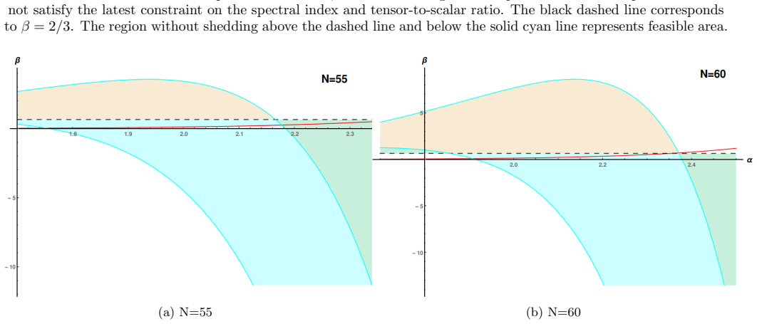
- [Section 2, Eq. (17); Section 4, Eq. (22); Section 6.3] The definition N ≡ ln(a_end/a(t)) in Eq. (17) fixes N = 0 at the end of inflation. Combining Eq. (22), ϵ_H = 3β/[2(N+1)^α], with the end condition ϵ_H = 1 at N = 0 forces β = 2/3 exactly. The paper instead infers only a lower bound β > 2/3 and then treats β as a free parameter, allowing values such as 0.67 < β < 3.75 for α = 2 in Section 6.3. For any β ≠ 2/3, the end of inflation occurs at N_end = (3β/2)^{1/α} − 1 ≠ 0, so N = 0 is not the end of inflation, and the integration in Eq. (26) that sets φ = φ_end at N = 0 is inconsistent. Consequently, the feasible regions in Figs. 8–14, the statement that 'we can find appropriate values of β' for 1.5 < α ≤ 2.2, and the LiteBIRD and CMB-S4 forecasts based on those regions are not well posed as a two-parameter model. A one-parameter version with β = 2/3 may still yield a similar α interval, but that is a different claim from the one presented.
- [Section 4, Eqs. (26)–(29)] The expressions for H(φ) in Eq. (28) and V(φ) in Eq. (29) omit the integration constant φ_end that Eq. (26) explicitly introduces. For example, for α = 2, Eq. (26) gives 1+N = exp[(φ − φ_end)/(√(3β) M_P)], so Eq. (27) yields H = H0 exp[−(3β/2) exp(−(φ − φ_end)/(√(3β) M_P))], not the φ_end-free expression in Eq. (28). The same omission occurs for general α and propagates into the supposedly exact potentials of Eq. (29). The paper must either keep φ_end throughout, or explicitly state that φ is measured from φ_end, and then correct Eqs. (28) and (29) accordingly. As written, the claim of deriving exact potentials is not supported.
- [Section 5, Eqs. (30)–(36); Section 8] The observable predictions n_S ≈ 1 − 3(1+ω) + d ln(1+ω)/dN and r ≈ 24(1+ω) are first-order slow-roll formulas, even though the paper emphasizes that the Hamilton-Jacobi formalism is more accurate. No numerical evolution or higher-order slow-roll computation is provided to validate these formulas across the full allowed parameter range. The slow-roll parameters are small at N = 55 for the region around β = 2/3, so the effect may be modest, but because the central result is a quantitative interval 1.50 < α ≤ 2.20, the paper should estimate the size of the neglected corrections or check the first-order expressions against exact numerical power spectra. The admission in Section 8 that 'we did not do rigorous numerical analysis' makes this validation necessary.
minor comments (5)
- [Section 2] There are several typographical errors, including 'flat FR W unverse' (should be 'universe') and 'tract' (should be 'track').
- [Section 4, after Eq. (22)] The sentence 'Considering these two we get a lower-bound of the parameter β > 2/3' should be 'β = 2/3' if N = 0 is the end of inflation; the distinction is not merely verbal, as it changes the number of free parameters.
- [Section 6.2] The sentence 'as β < 2/3 inflation goes on forever and model suffers from graceful exit problem' restates the end-of-inflation issue but should be reconciled with the definition of N; as written it contradicts the identification N = 0 with the end of inflation.
- [Figures 8–14] The red and cyan shaded regions in Figs. 8 and 9 are difficult to distinguish in grayscale; please use distinguishable hatching, line styles, or labels.
- [Eq. (29)] The typography of the exponents in the α = 1 and α = 2 entries of Eq. (29) should be checked carefully; several factors appear inconsistent with Eq. (28) unless φ_end is set to zero, which is not stated.
Circularity Check
End-of-inflation condition fixes β=2/3 by the paper's own definitions, so the claimed free-β viable regions are self-definitional artifacts; the α-window, the n_S–r relation, and the falsifiable LiteBIRD/CMB-S4 forecasts retain independent content.
-
self definitional
[Section 4 (Eqs. 19, 22; 'end of inflation' paragraph); applied in Section 6.3 (β range '0.67 < β < 3.75') and Section 8 (conclusion).]
"The end of inflation occurs naturally when ϵH = 1 and from the definition of e-foldings N = 0 at the end of inflation. Considering these two we get a lower-bound of the parameter β > 2/3, since β ≤ 2/3 would always imply ϵH < 1 and inflation goes on forever."
With N defined as e-folds remaining before the end (Eq. 17) and ϵH = 3β/[2(N+1)^α] (Eq. 22), the quoted end conditions (ϵH = 1, N = 0) give 3β/2 = 1, i.e. β = 2/3, not merely β > 2/3. The paper then treats β as free, claiming viable ranges such as '0.67 < β < 3.75' (Sec. 6.3) and 'we can find appropriate values of β' for 1.5<α≤2.2 (Abstract). For any β ≠ 2/3, ϵH(0) ≠ 1: β > 2/3 places exit at N = (3β/2)^{1/α} − 1 > 0, contradicting N's definition; β < 2/3 leaves N undefined. Eq. (26) ('φ = φend at N = 0'), the observables (35)-(36) at N = 50-60, and the β-viable regions in Figs. 8-14 are thus artifacts of the paper's own end-of-inflation construction, reducing the model as defined to β = 2/3.
full rationale
Most of the derivation chain is self-contained. From the parametrization 1+ω = β/(N+1)^α (Eq. 19) the paper derives ϵH (Eq. 22), the field evolution (Eqs. 23-26), the Hubble parameter (Eqs. 21, 27), and the implicit potential (Eqs. 28-29) purely algebraically within Hamilton-Jacobi formalism, with no observational input. The observable formulas (Eqs. 35-36) are substitutions into standard first-order relations (Eqs. 30-34) taken from the literature, and the consistency relation r/8 ≈ (1−n_S) − α/(1+N) (Eq. 37) is a genuine falsifiable constraint: it fails for α ≤ 1.5 and α ≥ 2.2. Constraining α and β from Planck 2018 and BICEP/Keck bounds is ordinary parameter estimation, not circularity, and the Section 7 forecasts are falsifiable in the proper sense: LiteBIRD/CMB-S4 non-detection of gravitational waves would rule out the parametrization. Self-citations (Refs. [18], [30], [33], [34]) provide background on EoS and Hamilton-Jacobi methods only and are not load-bearing; the present derivation is explicit. The one substantive issue is the self-definitional inconsistency flagged in the step: with N defined by Eq. (17) as e-folds remaining before the end, and with the end defined by ϵH = 1, Eq. (22) requires β = 2/3. The paper's 'β > 2/3' inference and subsequent use of β as an adjustable parameter in the viable regions (e.g., 0.67 < β < 3.75) do not respect its own definitions, so the claimed two-parameter freedom is an artifact. Because this flaw is confined to the β-freedom framing — the α-window and the qualitative rule-out forecast survive the β = 2/3 fix — the circularity is partial rather than total. Slow-roll validity over the full parameter range is a correctness risk, not a circularity issue, and receives no separate circularity weight.
Assumptions & free parameters
free parameters (2)
- α =
1.5 < α ≤ 2.2 (for N=55)
- β =
Range depends on α and N; e.g., for α=2 and N=55, 0.67 < β < 3.75
assumptions (4)
- domain assumption The universe during inflation is described by a flat FRW metric with a homogeneous scalar field.
- domain assumption The Hamilton-Jacobi formalism provides an exact description of the background inflationary dynamics.
- domain assumption The first-order slow-roll approximations for n_S and r, Eqs. (30)-(34), are valid.
- ad hoc to paper The parametrization 1+ω = β/(N+1)^α is the model to be tested.
Cite this review
Pith. "Pith review of Returning Back to Mukhanov Parametrization of Inflationary Equation of State." pith.science (2026). https://pith.science/paper/YSGQYRR6
@misc{pith2026241216703,
  author       = {Pith},
  title        = {Pith review of: Returning Back to Mukhanov Parametrization of Inflationary Equation of State},
  year         = {2026},
  howpublished = {\url{https://pith.science/paper/YSGQYRR6}},
  note         = {Machine review of arXiv:2412.16703}
}
abstract
We have re-examined Mukhanov parametrization for inflationary equation of state, $1+\omega=\frac{\beta}{({N}+1)^\alpha}$, in the light of Planck 2018 results and latest bound of tensor-to-scalar ratio employing Hamilton-Jacobi formalism. We have found that the current observational values of scalar spectral index and tensor-to-scalar ratio can be used efficiently to constrain the model parameters. The recent bound of $r<0.032$ has been used to put an upper bound on one of the model parameter. Whereas 1-$\sigma$ bound of the scalar spectral index $0.9607\leq n_{_S}\leq 0.9691$ along with the upper bound of tensor-to-scalar ratio provided restriction on the other model parameter $1.50<\alpha\leq2.20$. These bounds however depend on the number of e-foldings still left before the end of inflation and whenever $1.50<\alpha\leq2.20$ we can find appropriate values of the other model parameter $\beta$ so that the observational predictions are in tune with the latest available inflationary observables. We have further utilized the predictions from forthcoming CMB missions in the likes of CMB-S4 and LiteBIRD in order to obtain bounds on the model parameters. We find that detection of gravity waves would help us constrain the model parameters further. But in the absence of detection of primordial gravity wave signal by these CMB missions may rule out Mukhanov parametrization.
Figures


Figures from the paper (11 more)


Reference graph
Works this paper leans on
-
[1]
Returning Back to Mukhanov Parametrization of Inflationary Equation of State
INTRODUCTION Cosmic inflation, by far the best bet for early universe scenario, has started its journey more than four decades ago in order to figure out the Big Bang puzzles. It has resolved the problems of Big Bang theory in a very elegant way. Not only that, inflation has surprised us by supplying quantum seeds for cosmological fluctuations observed in...
work page Pith review arXiv 2025
-
[2]
HAMIL TON JACOBI FORMALISM The most commonly used tool to solve the inflationary dynamics is the slow-roll approximations [22]. But the need to go beyond slow-roll approximation is slowly but steadily licking in considering the ever increasing level of precision of the present telescopes. To incorporate all the models irrespective of slow-roll approximati...
-
[3]
MUKHANOV P ARAMETRIZA TION Inflationary paradigm has been investigated recently through the parametrization of inflationary Equation-of-State (EoS henceforth) as a function of number of e-foldings, N . The main motivation was to develop a model independent framework for the investigation and confrontation of cosmic inflation with recent observations, and ...
-
[4]
FROM EOS TO INFLA TIONAR Y POTENTIAL Since inflation is a high energy phenomena, working with a specific form of the potential directly establishes the link with high energy physics. Whereas EoS formalism helps us obtain observational predictions at ease without going into the details of underlying physics. Now we shall see in the following analysis that ...
-
[5]
FROM EOS TO INFLA TIONAR Y OBSER V ABLES Considering N as new time variable it is possible to express all the inflationary observables in terms of the EoS [12, 37], which up to the first order in slow-roll parameters are given by nS ≃ 1 − 3 (1 +ω) + d dN ln (1 +ω) (30) αS ≃ 3 d dN (1 + ω) − d2 dN 2 ln (1 +ω) (31) r ≃ 24 (1 +ω) (32) nT ≃ −3 (1 +ω) (33) αT ...
-
[6]
INFLA TIONAR Y MODELS In this section we shall investigate few inflationary models by fixing the model parameter, α. In Fig.1 we have plotted the inflationary potentials for different values of the model parameter α and for four values of β in logarithmic scale. From the figure it is very clear that the potential has adequate flat region which is required...
work page 2018
-
[7]
The forthcoming ground based CMB-S4 [6] mission along with space mission LiteBird
MUKHANOV P ARAMETRIZA TION AND FUTURE CMB MISSIONS Since the detection of gravity waves by LIGO and Virgo scientific collaboration [40, 41], we are eagerly waiting for the detection of large-scale primordial gravity waves through the CMB B-mode polarization, which are supposed to be produced during inflation. The forthcoming ground based CMB-S4 [6] missio...
-
[8]
are expected to detect inflationary gravity waves provided r >0.003 or will set an upper-bound r <0.001 [42, 43] in the absence of detection. In the context of upcoming CMB missions LiteBIRD and CMB-S4 we shall shed light on the parameter space for two free parameters, α, β, in the following. 7.1. LiteBIRD LiteBIRD, the Lite (Light) satellite for the stud...
Show all 54 references
-
[9]
CONCLUSION In this article we have reviewed the prospects and consequences of Mukhanov Parametrization of inflationary paradigm through the equation of state formalism employing Hamilton-Jacobi formulation. We have seen that the initial claim of model independent study of infl...
-
[10]
Akrami, F
Y. Akrami, F. Arroja, M. Ashdown, J. Aumont, C. Baccigalupi, M. Ballardini, A. J. Banday, R. Barreiro, N. Bartolo, S. Basak, et al., Astronomy & Astrophysics 641, A10 (2020)
2020
-
[11]
Aghanim, Y
N. Aghanim, Y. Akrami, M. Ashdown, J. Aumont, C. Baccigalupi, M. Ballardini, A. Banday, R. Barreiro, N. Bartolo, S. Basak, et al., Astronomy & Astrophysics 641, A6 (2020)
2020
-
[12]
P. A. Ade, N. Aghanim, C. Armitage-Caplan, M. Arnaud, M. Ashdown, F. Atrio-Barandela, J. Aumont, C. Baccigalupi, A. J. Banday, R. Barreiro, et al., Astronomy & Astrophysics 571, A22 (2014)
2014
-
[13]
D. N. Spergel et. al., Astrophys. J. Suppl. 170, 377 (2007)
2007
-
[14]
P. Ade, Z. Ahmed, R. Aikin, K. Alexander, D. Barkats, S. Benton, C. Bischoff, J. Bock, R. Bowens-Rubin, J. Brevik, et al., Physical review letters 121, 221301 (2018)
2018
-
[15]
K. N. Abazajian et al., arXiv preprint arXiv:1610.02743 (2016)
2016 arXiv
-
[16]
Matsumura, Y
T. Matsumura, Y. Akiba, J. Borrill, Y. Chinone, M. Dobbs, H. Fuke, A. Ghribi, M. Hasegawa, K. Hattori, M. Hattori, et al., Journal of Low Temperature Physics 176, 733 (2014)
2014
-
[17]
Vagnozzi and A
S. Vagnozzi and A. Loeb, The Astrophysical Journal Letters 939, L22 (2022)
2022
-
[18]
Mukhanov, EPJC 73, 2486 (2013)
V. Mukhanov, EPJC 73, 2486 (2013)
2013
-
[19]
Martin, C
J. Martin, C. Ringeval, and V. Vennin, Physics of the Dark Universe 5, 75 (2014)
2014
-
[20]
Roest, Journal of Cosmology and Astroparticle Physics 2014, 007 (2014)
D. Roest, Journal of Cosmology and Astroparticle Physics 2014, 007 (2014)
2014
-
[21]
Garcia-Bellido and D
J. Garcia-Bellido and D. Roest, PRD 89, 103527 (2014)
2014
-
[22]
Barranco, L
L. Barranco, L. Boubekeur, and O. Mena, Physical Review D 90, 063007 (2014)
2014
-
[23]
Bamba, S
K. Bamba, S. Nojiri, S. D. Odintsov, and D. Saez-Gomez, Physical Review D 90, 124061 (2014)
2014
-
[24]
Bamba, S
K. Bamba, S. Nojiri, and S. D. Odintsov, Physics Letters B 737, 374 (2014)
2014
-
[25]
Boubekeur, E
L. Boubekeur, E. Giusarma, O. Mena, and H. Ram ´ ırez, Physical Review D91, 083006 (2015)
2015
-
[26]
Gariazzo, O
S. Gariazzo, O. Mena, H. Ramirez, and L. Boubekeur, Physics of the dark universe 17, 38 (2017)
2017
-
[27]
B. K. Pal, IJMPD 32, 2350019 (2023)
2023
-
[28]
Martin, in The Cosmic Microwave Background(Springer, 2016), pp
J. Martin, in The Cosmic Microwave Background(Springer, 2016), pp. 41–134
2016
-
[29]
A. D. Linde, PLB 108, 389 (1982)
1982
-
[30]
Albrecht and P
A. Albrecht and P. J. Steinhardt, PRL 48, 1220 (1982)
1982
-
[31]
A. R. Liddle, P. Parsons, and J. D. Barrow, PRD 50, 7222 (1994)
1994
-
[32]
Garc ´ ıa-Bellido and D
J. Garc ´ ıa-Bellido and D. Wands, PRD54, 7181–7185 (1996)
1996
-
[33]
Muslimov, CQG 7, 231 (1990)
A. Muslimov, CQG 7, 231 (1990)
1990
-
[34]
Salopek and J
D. Salopek and J. Bond, PRD 42, 3936 (1990)
1990
-
[35]
J. E. Lidsey, A. R. Liddle, E. W. Kolb, E. J. Copeland, T. Barreiro, and M. Abney, RMP 69, 373 (1997)
1997
-
[36]
Ade et al., PRL 127, 151301 (2021)
P. Ade et al., PRL 127, 151301 (2021)
2021
-
[37]
Tristram et al., PRD 105, 083524 (2022)
M. Tristram et al., PRD 105, 083524 (2022)
2022
-
[38]
Kinney, PRD 56, 2002 (1997)
W. Kinney, PRD 56, 2002 (1997)
1997
-
[39]
B. K. Pal, S. Pal, and B. Basu, JCAP 04, 009 (2012)
2012
-
[40]
Videla, EPJC 77, 142 (2017)
N. Videla, EPJC 77, 142 (2017)
2017
-
[41]
B. K. Pal, EPJC 78, 358 (2018)
2018
-
[42]
B. K. Pal, S. Pal, and B. Basu, JCAP 01, 029 (2010)
2010
-
[43]
B. K. Pal, S. Pal, and B. Basu, IJMPD 21, 1250017 (2012)
2012
-
[44]
W. H. Kinney, Physical Review D 66, 083508 (2002)
2002
-
[45]
E. J. Copeland, A. R. Liddle, and D. Wands, Phys. Rev. D 57, 4686–4690 (1998)
1998
-
[46]
V. F. Mukhanov, Physical Foundations of Cosmology(Cambridge University Press, 2005)
2005
-
[47]
A. D. Linde, PLB 129, 177 (1983)
1983
-
[48]
A. D. Linde, JETP Lett. 38, 176 (1983)
1983
-
[49]
B. P. Abbott et al., PRL 116, 061102 (2016)
2016
-
[50]
B. P. Abbott et al., PRL 116, 241103 (2016)
2016
-
[51]
Abazajian, G
K. Abazajian, G. E. Addison, P. Adshead, Z. Ahmed, D. Akerib, A. Ali, S. W. Allen, D. Alonso, M. Alvarez, M. A. Amin, et al., The Astrophysical Journal 926, 54 (2022)
2022
-
[52]
Belkner, J
S. Belkner, J. Carron, L. Legrand, C. Umilt` a, C. Pryke, C. Bischoff, C.-S. Collaboration, et al., The Astrophysical Journal 964, 148 (2024)
2024
-
[53]
Collaboration, E
L. Collaboration, E. Allys, K. Arnold, J. Aumont, R. Aurlien, S. Azzoni, C. Baccigalupi, A. Banday, R. Banerji, R. Barreiro, et al., Progress of Theoretical and Experimental Physics 2023, 042F01 (2023). 17
2023
-
[54]
Ghigna, A
T. Ghigna, A. Adler, K. Aizawa, H. Akamatsu, R. Akizawa, E. Allys, A. Anand, J. Aumont, J. Austermann, S. Azzoni, et al., arXiv preprint arXiv:2406.02724 (2024)
2024 arXiv
Reviewed August 11, 2026 · model on record in the stance chip above.
Discussion (0). Continue with ORCID to comment.