Overcoming the low signal-to-noise problem for hybrid mode-selective photonic lantern-based wavefront correction using machine learning

Adam K Taras; Akira Rodziewicz-Ryan; Barnaby Norris; Christopher H Betters; Daniel S Dahl; Frantz Martinache; Jin Wei; Julia J Bryant; Marc-Antoine Martinod; Nathan K Long

REVIEW 3 major objections 4 minor 20 references

In simulation, a transformer neural network that reads the previous 50 lantern-core intensity measurements estimates temporally correlated wavefronts better than a single-frame convolutional network, cutting residual tip/tilt error to 0.05

Reviewed by Pith at T0; open to challenge. T0 means a machine referee read the full paper against a public rubric. the ladder, T0–T4 →

Challenge this review Re-run · record.json Download PDF Read on arXiv ↗

T0 review · deepseek-v4-flash

2026-08-03 01:57 UTC pith:YUKUJEB2

load-bearing objection First transformer-for-lantern-wavefront-sensing benchmark, but the reported TNN advantage is currently an unequal-information artifact — the CNN gets one frame, the TNN gets fifty. the 3 major comments →

arxiv 2607.03285 v2 pith:YUKUJEB2 submitted 2026-07-03 physics.optics astro-ph.IMphysics.ins-det

Overcoming the low signal-to-noise problem for hybrid mode-selective photonic lantern-based wavefront correction using machine learning

Nathan K Long , Barnaby Norris , Daniel S Dahl , Christopher H Betters , Julia J Bryant , Nick Cvetojevic , Sergio Leon-Saval , Frantz Martinache

show 5 more authors

Marc-Antoine Martinod Akira Rodziewicz-Ryan Adam K Taras Jin Wei Peter G Tuthill

This is my paper

classification physics.optics astro-ph.IMphysics.ins-det

keywords photonic lanternwavefront sensingadaptive opticstransformer neural networkconvolutional neural networktip/tilt aberrationVon Kármán turbulenceStrehl ratio

verification ladder T0 review T1 audit T2 compute T3 formal T4 reserved

The pith

A machine-rendered reading of the paper's core claim, the machinery that carries it, and where it could break.

The paper asks whether a neural network can estimate wavefront corrections from the dim sensing cores of a hybrid mode-selective photonic lantern, where most light is reserved for the science channel. It compares a convolutional network that sees one snapshot of core intensities with a transformer network that sees the previous 50 time steps. On simulated tip/tilt and Von Kármán seeing, the transformer improves temporally correlated wavefront estimates, while the two networks perform about the same on independent random wavefronts. The authors read this as evidence that temporal machine learning can help address the signal-to-noise trade-off inherent to lantern-based wavefront sensing.

Core claim

On simulated data for a six-core hybrid mode-selective photonic lantern, the transformer neural network reduces residual temporal tip/tilt RMS error to 0.05 rad from 0.07 rad for the convolutional network, and increases mean temporal Von Kármán Strehl ratio from about 0.29 to about 0.36. For randomized, uncorrelated wavefronts the two architectures perform nearly identically, which isolates the temporal advantage: self-attention over the previous 50 lantern intensity measurements lets the transformer exploit correlations in how the wavefront evolves, something a one-shot CNN cannot do.

What carries the argument

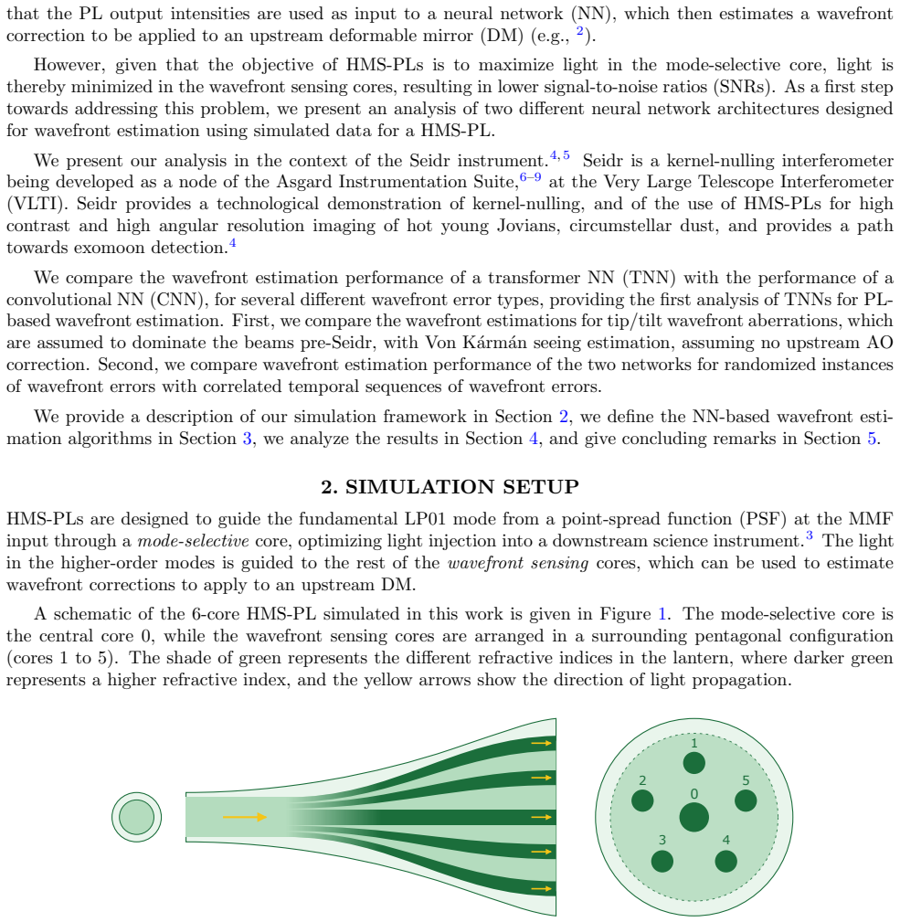
The central objects are a six-core hybrid mode-selective photonic lantern (a fiber device that sends the fundamental optical mode to a central science core and distributes the remaining light among five surrounding sensing cores) and the transfer matrix that maps its six guided LP modes (linear-polarized fiber modes) to the output core intensities. On top of that, the transformer neural network — a machine-learning model that weighs which past time steps matter via self-attention — reads a sequence of lantern intensity vectors and estimates the current wavefront, whereas the convolutional network, which finds spatial patterns in image-like arrays, sees only a single intensity vector.

Load-bearing premise

The simulation assumes a six-mode lantern transfer matrix computed by finite-difference beam propagation, with noiseless intensity measurements and no validation against a fabricated device; if the real lantern couples modes differently, carries more modes, or adds noise, the reported transformer advantage may not survive.

What would settle it

Train the same CNN and transformer on lantern intensities recorded from a fabricated six-core hybrid mode-selective photonic lantern in the laboratory, with controlled input wavefronts, and compare residual wavefront error against the simulation values; if the transformer's temporal margin disappears or absolute errors exceed 0.05 rad, the simulated transfer matrix is the likely point of failure. A cheaper computational check is to rerun the study with a transfer matrix from a different lantern geometry or with more than six guided modes.

Watch this falsifier — get emailed when new claim-graph text bears on it.

If this is right

If the temporal advantage holds outside simulation, transformer-based predictors could let a lantern reserve more light for the science channel while still sensing wavefronts from dimmer cores.
The small residual errors (0.05 rad for temporal tip/tilt) suggest that low-order wavefront correction from a six-core lantern is feasible in the regime Seidr is expected to encounter.
Because both networks act as low-pass filters on Von Kármán wavefronts, a six-core lantern can only correct low-order errors; higher-order correction would require a lantern supporting more modes.
The transformer's sequential latency (about 0.7 ms on one GPU) is larger than the CNN's, so closed-loop use will depend on whether that latency stays within the AO control budget.
The same temporal-attention approach is a natural candidate for closed-loop predictive adaptive optics, where the network would estimate not just the current wavefront but the correction needed after loop delay.

Where Pith is reading between the lines

These are editorial extensions of the paper, not claims the author makes directly.

The paper frames the work as a step toward the low-SNR problem, but the simulation itself adds no photon or detector noise; a direct extension is to test whether the transformer's temporal advantage survives photon-starved intensities.
Because the temporal sequences are generated from smoothed Gaussian random walks under a frozen-flow assumption, retraining on actual adaptive-optics residual telemetry would test whether the temporal margin is an artifact of the simulated correlations.
The transfer matrix is the load-bearing physical model; measuring a fabricated lantern's intensity response and comparing it to the simulation would show whether this network can be trusted in hardware.

Editorial analysis

A structured set of objections, weighed in public.

Desk editor's note, referee report, simulated authors' rebuttal, and a circularity audit.

Desk Editor's Note

First transformer-for-lantern-wavefront-sensing benchmark, but the reported TNN advantage is currently an unequal-information artifact — the CNN gets one frame, the TNN gets fifty.

read the letter

Quick take: this is a clean simulation study that asks a fair question — can a transformer use temporal sequences of photonic-lantern intensities to predict wavefront corrections better than a CNN — and the answer it reports is not yet supported because the two networks were given different information. The TNN sees the previous 50 intensity vectors; the CNN sees only the current one. So the headline 0.05 vs 0.07 rad residual, or 0.36 vs 0.29 Strehl, tells you something about having 50 frames of context, not about transformers being better at temporal structure. Any model that took 50 frames as input (a concatenating MLP, a temporal CNN, even a persistence predictor) might do the same. The paper needs an equal-information baseline — same input frame count for both architectures, plus a previous-frame persistence baseline — before the architectural claim can be taken seriously.

The title's 'low signal-to-noise' framing is also untested: no noise is added to the lantern intensities at all. The simulation is noiseless, so the SNR trade-off the abstract promises is left entirely to future work.

What the paper does well: it is clearly written, the simulation chain is sensible (Fraunhofer propagation, LP-mode projection, transfer matrix from a beam-propagation method), the hyperparameters are reported, and the authors are honest about the low-order limits of a 6-core lantern. The application to Seidr and Asgard is real and timely. The first use of a transformer for lantern wavefront sensing is worth recording, even if the demonstration here is preliminary.

Secondary concerns: the transfer matrix is simulated, not measured against a fabricated device, and only six LP modes are retained — a real lantern will have mode-dependent loss, phase errors, and possibly more modes. That is acceptable for a first exploration, but it should be said more forcefully. The Von Karman parameters (r0 = 0.4 m, L0 = 10 m) look arbitrary. There are no error bars or repeated seeds, so the 0.02 rad difference could be noise. Minor: the temporal Zernike coefficients are generated by smoothing Gaussian noise, which is a reasonable stand-in but not real AO residual telemetry.

Bottom line: the paper is worth engaging with for the Seidr team and anyone working on PL wavefront sensing. It deserves peer review, but the referee should send it back for a corrected comparison. If an equal-information baseline still shows a TNN advantage, that would be a genuinely useful result. As it stands, I wouldn't cite the headline claim.

Referee Report

3 major / 4 minor

Summary. The paper presents a simulation study of a 6-core hybrid mode-selective photonic lantern (HMS-PL) as a wavefront sensor for the Seidr instrument at VLTI. The authors simulate wavefront-distorted PSFs, propagate the complex field through the lantern's LP modes using a BPM-derived transfer matrix, and train two neural networks—a convolutional neural network (CNN) and a transformer neural network (TNN)—to estimate the input wavefront from the measured core intensities. They compare performance for random and temporal tip/tilt aberrations and for Von Kármán turbulence, reporting that the TNN outperforms the CNN in the temporal cases: residual tip/tilt RMS error of 0.05 rad versus 0.07 rad and mean Strehl ratio of 0.36 versus 0.29 (Section 4, Figures 5–6). The authors interpret this as evidence that transformer architectures are promising for temporal photonic-lantern wavefront estimation.

Significance. If the claimed advantage of the TNN over the CNN were properly established, the result would be of practical interest for photonic-lantern wavefront sensing in interferometric instruments like Seidr, and could motivate further work on predictive AO with lantern sensors. The paper also demonstrates a useful simulation pipeline for a realistic lantern geometry and provides clear architectural descriptions and training details. However, the central comparative claim is currently undermined by an uncontrolled variable: the TNN receives 50 previous intensity measurements while the CNN receives only the current measurement (Section 3.3). The results are therefore evidence that temporal context helps, not that transformer attention is the reason. The title's 'low signal-to-noise' framing is likewise untested because all simulations are noiseless. These issues are load-bearing for the paper's main conclusions.

major comments (3)

[Section 3.3 and Section 4.1] The core TNN-vs-CNN comparison is confounded. In Section 3.3 the authors state that for temporal phase screens 'the CNN takes a single lantern intensity measurement as input, while the TNN takes the previous M_t = 50 lantern intensity measurements as input.' Thus the TNN has access to 50× more information, including the temporal context that the CNN is explicitly denied. The reported advantage in Section 4.1 (0.05 vs 0.07 rad RMS) and Section 4.2 (Strehl 0.36 vs 0.29) therefore conflates architecture with input length. Any sequence-aware model, including a CNN with a 1D temporal kernel or an MLP on the concatenated 50-frame sequence, might show the same benefit. The conclusion in Section 5 that a TNN 'outperforms' a CNN at temporal wavefront estimation is not supported without an equal-information baseline. I recommend adding baselines where all models receive the same temporal context (
[Section 2 and Section 4] The paper's title and abstract emphasize the 'low signal-to-noise' problem, and the Introduction frames the work as a first step toward addressing the SNR trade-off. However, the simulations are completely noiseless: the lantern intensities are computed deterministically from the transfer matrix, and no photon noise, read noise, or other detector noise is added anywhere in Section 2 or in the training/operation described in Section 3.3. Consequently, the reported RMS errors and Strehl ratios are for a noise-free idealization, and no conclusion can be drawn about how the CNN or TNN would perform under reduced light in the wavefront-sensing cores. This is a central mismatch between the stated motivation and the actual experiments. The authors should either add a noise model with varying SNR (e.g., Poisson noise on the core intensities) or explicitly state that the SNR question is deferred
[Section 2, transfer matrix and mode truncation] The fidelity of the simulated lantern is a significant uncertainty. The transfer matrix in Figure 2 is obtained from a finite-difference beam propagation method for a specific design, and the decomposition in Eq. (1) retains only six LP modes. There is no validation against a fabricated lantern or laboratory measurement for this Seidr design, and the authors note in Section 2.1 that the six-mode lantern 'only provides a low-order wavefront sensing capability.' If the physical lantern couples modes differently, or if higher-order modes carry non-negligible power, the intensity-to-wavefront mapping learned by the networks will not match the real instrument. A robustness test—e.g., perturbing the transfer matrix, adding a seventh mode, or training on a measured matrix—would substantially strengthen the claims. As it stands, the numerical results are tied to the accuracy of one simulated tra

minor comments (4)

[General] There are several typographical issues: 'V alue' and 'T ransformer' in the tables/section headings, and inconsistent spacing around Greek letters. These should be corrected in a final revision.
[Section 4.1] The text says both networks 'reduce the mean tip/tilt RMS error by nearly an order of magnitude.' With uncorrected 0.50 rad and post-correction 0.07 rad, the reduction is roughly 7×, which is close to one order of magnitude; for the random TNN case (0.08 rad) it is about 6×. This is acceptable but could be phrased more precisely.
[Section 4.2] The Strehl ratio is computed using the Maréchal approximation in Eq. (6). It would be helpful to state explicitly that this approximation is used for the reported Strehl values, including the uncorrected wavefronts, since the approximation is only accurate for small phase variance.
[References] Reference [5] is cited as 'SPIE (2026)' while the paper appears to be from 2026; please double-check that all reference years and proceedings identifiers are consistent and correct.

Circularity Check

0 steps flagged

No significant circularity: the supervised-learning simulation is self-contained, and the TNN-vs-CNN comparison is not forced by construction or by the authors' prior work.

full rationale

The paper's claimed result is an empirical machine-learning comparison, not an analytical derivation. The pipeline is: simulated phase screens -> Fraunhofer PSF -> LP-mode decomposition (Eq. 1) -> fixed 6-core lantern transfer matrix computed by finite-difference beam propagation (Section 2, Refs 10-11) -> neural-network training on a 70k/15k/15k split with held-out test data. The transfer matrix is computed by an external numerical method, not fitted to the NN outputs, and the NN outputs are evaluated against ground-truth wavefronts that were not used in training. No equation is defined in terms of the quantity it is used to predict, and no fitted parameter is relabeled as a prediction. The authors' self-citations (Refs 2-5, 15, 20) supply device context, earlier ML for lanterns, and on-sky PL demonstrations, but none functions as a uniqueness theorem, ansatz, or load-bearing premise that determines the TNN result; the TNN-vs-CNN comparison is new and has independent content. The paper's main weaknesses—unequal temporal input length (50 frames for TNN vs 1 frame for CNN, Section 3.3) and the unvalidated simulated 6-mode lantern—are confounds and external-validity concerns, not circular reductions. They do not make the result equivalent to its inputs by construction. Therefore, under the quoting/reduction standard, no circularity step is present.

Axiom & Free-Parameter Ledger

6 free parameters · 8 axioms · 0 invented entities

The paper introduces no new physical entities. The central claim rests on a chain of simulation and modeling assumptions: the Von Kármán atmosphere model, frozen-flow temporal evolution, the BPM-derived 6-mode transfer matrix, noiseless intensities, and a fixed set of NN hyperparameters. Several of these are unvalidated against the physical Seidr lantern, and the temporal-context length M_t is the key free parameter behind the headline TNN advantage.

free parameters (6)

Fried parameter r0 and outer scale L0 = r0=0.4 m, L0=10 m
Chosen values for Von Kármán seeing generation (Section 2.1). They set the difficulty of the seeing cases and hence affect all Strehl results.
Transverse wind speed = 10 m/s
Used with Taylor frozen flow to generate temporal sequences (Section 2.1).
RMS tip/tilt error = 100 nm
Chosen scale for tip/tilt wavefront errors (Section 2.1).
Gaussian smoothing kernel width for temporal Zernike coefficients = not specified
The temporal sequences convolve a Gaussian kernel with Gaussian noise, but the kernel width is not reported. This affects temporal correlation length and the TNN's advantage.
TNN temporal context length M_t = 50
The TNN receives 50 previous intensity measurements while the CNN receives only one (Section 3.3). This is the main confound in the central comparison and is not swept or ablated.
NN hyperparameters = dm=128, dff=256, heads=4, layers=2; CNN filters=64, dense=128, blocks=4
Chosen architecture hyperparameters in Tables 2 and 3. No hyperparameter optimization is performed, so the comparison may depend on these fixed choices.

axioms (8)

standard math Fraunhofer diffraction models the PSF at the lantern input
Section 2 assumes Fraunhofer propagation from the telescope aperture to the focal plane.
domain assumption Von Kármán PSD describes atmospheric phase statistics
Equation (2) is used to generate phase screens; the validity of this model for the VLTI site is assumed.
domain assumption Taylor frozen-flow hypothesis generates realistic temporal phase sequences
Section 2.1 uses a frozen-flow wind speed of 10 m/s to evolve phase screens; real AO residuals may have different temporal statistics.
domain assumption The 6-core HMS-PL guides exactly six LP modes and the BPM transfer matrix accurately represents the physical lantern
Section 2 and Figure 2 use a BPM-computed transfer matrix with six LP modes; no laboratory validation is provided for this Seidr-specific lantern.
domain assumption Seidr wavefront errors are dominated by tip/tilt
Section 2.1 assumes the dominant aberrations after upstream AO are tip/tilt; the relevance of the tip/tilt experiments depends on this.
ad hoc to paper Simulated lantern intensities are noiseless
Despite the title's SNR focus, no photon or detector noise is added to the intensities used for training or testing. This omission is not flagged in the simulation description.
domain assumption Neural networks can learn the lantern-intensity-to-wavefront mapping from supervised training
Standard supervised-learning assumption in Section 3.3, supported by prior PL-ML work.
standard math Maréchal approximation S≈exp(-σ²) is valid for Strehl estimation
Equation (6) is used to convert residual wavefront variance to Strehl ratio.

pith-pipeline@v1.3.0-alltime-deepseek · 8357 in / 12435 out tokens · 132926 ms · 2026-08-03T01:57:59.817956+00:00 · methodology

0 comments

read the original abstract

Hybrid mode-selective photonic lanterns transform an input complex point-spread function into several single-mode outputs, where a selected core feeds the fundamental mode to a photonic science instrument, while the remaining cores are used for wavefront sensing in a closed-loop adaptive optics system. A neural network maps the intensities of the wavefront sensing cores to an estimated wavefront correction, which is applied to an upstream deformable mirror. However, there exists a trade between maximizing the amount of light reserved for the photonic instrument and the reduced signal-to-noise ratios for the wavefront sensing cores. We explore wavefront correction for the Seidr instrument, a part of the Asgard Suite for the Very Large Telescope Interferometer. We evaluate different neural network architectures, comparing wavefront estimation performance for different wavefront error types, as a first step toward addressing the signal-to-noise trade-off. Results show transformer neural networks as a promising solution for temporal photonic lantern-based wavefront estimation.

Figures

Figures reproduced from arXiv: 2607.03285 by Adam K Taras, Akira Rodziewicz-Ryan, Barnaby Norris, Christopher H Betters, Daniel S Dahl, Frantz Martinache, Jin Wei, Julia J Bryant, Marc-Antoine Martinod, Nathan K Long, Nick Cvetojevic, Peter G Tuthill, Sergio Leon-Saval.

**Figure 1.** Figure 1: Schematic of a 6-core hybrid mode-selective photonic lantern. [PITH_FULL_IMAGE:figures/full_fig_p002_1.png] view at source ↗

**Figure 2.** Figure 2: Convolutional neural network architecture designed for hybrid mode-selective photonic lantern wavefront esti [PITH_FULL_IMAGE:figures/full_fig_p005_2.png] view at source ↗

**Figure 2.** Figure 2: 6-core hybrid mode-selective photonic lantern intensity (left) and phase (right) transfer matrices for [PITH_FULL_IMAGE:figures/full_fig_p003_2.png] view at source ↗

**Figure 3.** Figure 3: TNN architecture designed for hybrid mode-selective photonic lantern wavefront estimation. Sequence of [PITH_FULL_IMAGE:figures/full_fig_p006_3.png] view at source ↗

**Figure 3.** Figure 3: Convolutional neural network architecture designed for hybrid mode-selective photonic lantern wavefront esti [PITH_FULL_IMAGE:figures/full_fig_p005_3.png] view at source ↗

**Figure 4.** Figure 4: Tip/tilt wavefront aberration RMS error before and after wavefront estimation. [PITH_FULL_IMAGE:figures/full_fig_p007_4.png] view at source ↗

**Figure 4.** Figure 4: TNN architecture designed for hybrid mode-selective photonic lantern wavefront estimation. Sequence of [PITH_FULL_IMAGE:figures/full_fig_p006_4.png] view at source ↗

**Figure 5.** Figure 5: Strehl ratio probability density functions (PDFs) for Von K´arm´an seeing, both with randomized and sequential [PITH_FULL_IMAGE:figures/full_fig_p008_5.png] view at source ↗

**Figure 6.** Figure 6: Example wavefronts for temporal Von K´arm´an seeing, uncorrected and after wavefront estimation using the [PITH_FULL_IMAGE:figures/full_fig_p009_6.png] view at source ↗

**Figure 7.** Figure 7: Example wavefronts for temporal Von K´arm´an seeing, uncorrected and estimated using the TNN and CNN. [PITH_FULL_IMAGE:figures/full_fig_p009_7.png] view at source ↗

Review history (2 revisions) →

discussion (0)

Reference graph

Works this paper leans on

20 extracted references · 1 linked inside Pith

[1]

Photonic lanterns,

Leon-Saval, S. G., Argyros, A., and Bland-Hawthorn, J., “Photonic lanterns,”Nanophotonics2(5-6), 429– 440 (2013)

2013
[2]

An all-photonic focal-plane wavefront sensor,

Norris, B. R., Wei, J., Betters, C. H., Wong, A., and Leon-Saval, S. G., “An all-photonic focal-plane wavefront sensor,”Nature Communications11(1), 5335 (2020)

2020
[3]

Optimal broad- band starlight injection into a single-mode fibre with integrated photonic wavefront sensing,

Norris, B., Betters, C., Wei, J., Yerolatsitis, S., Amezcua-Correa, R., and Leon-Saval, S., “Optimal broad- band starlight injection into a single-mode fibre with integrated photonic wavefront sensing,”Optics Ex- press30(19), 34908–34917 (2022)

2022
[4]

Kernel nulling at VLTI with photonic lanterns for optimal fibre injection,

Taras, A. K., Norris, B., Chhabra, S., Cvetojevic, N., Foriel, V., Ireland, M., Kraus, S., Leon-Saval, S., Martinache, F., Paul, J., et al., “Kernel nulling at VLTI with photonic lanterns for optimal fibre injection,” in [Optical and Infrared Interferometry and Imaging IX],13095, 242–250, SPIE (2024)

2024
[5]

Seidr update: photonic ‘black magic’ for high-contrast interferometry using kernel-nulling and photonic lanterns,

Long, N. K., Dahl, D. S., Betters, C. H., Bryant, J. J., Cvetojevic, N., Ireland, M. J., Kraus, S., Leon-Saval, S., Martinache, F., Martinod, M.-A., Norris, B., Paul, J., Rodziewicz-Ryan, A., Taras, A. K., Wei, J., and Tuthill, P. G., “Seidr update: photonic ‘black magic’ for high-contrast interferometry using kernel-nulling and photonic lanterns,” in [Op...

2026
[6]

High-angular resolution and high contrast observations from Y to L band at the Very Large Telescope Interferometer with the Asgard Instrumental suite,

Martinod, M.-A., Defr` ere, D., Ireland, M., Kraus, S., Martinache, F., Tuthill, P., Bigioli, A., Bouzerand, E., Bryant, J., Chhabra, S., et al., “High-angular resolution and high contrast observations from Y to L band at the Very Large Telescope Interferometer with the Asgard Instrumental suite,”Journal of Astronomical Telescopes, Instruments, and System...

2023
[7]

Heimdallr, Baldr, and Solarstein: designing the next generation of VLTI instruments in the Asgard suite,

Taras, A. K., Robertson, J. G., Allouche, F., Courtney-Barrer, B., Carter, J., Crous, F., Cvetojevic, N., Ireland, M., Lagarde, S., Martinache, F., et al., “Heimdallr, Baldr, and Solarstein: designing the next generation of VLTI instruments in the Asgard suite,”Applied Optics63(14), D41–D49 (2024)

2024
[8]

Baldr: a Zernike wavefront sensor for VLTI/Asgard,

Courtney-Barrer, B., Robertson, G., Taras, A., Bernard, J. T., McGuinness, G., Crous, F., Tuthill, P., N’Diaye, M., Langford, C., Cvetojevic, N., et al., “Baldr: a Zernike wavefront sensor for VLTI/Asgard,” in [Adaptive Optics Systems IX],13097, 362–375, SPIE (2024)

2024
[9]

Asgard/NOTT: L-band nulling interferometry at the VLTI. II. Warm optical design and injection system,

Garreau, G., Bigioli, A., Laugier, R., Raskin, G., Morren, J., Berger, J.-P., Dandumont, C., Goldsmith, H.- D. K., Gross, S., Ireland, M., et al., “Asgard/NOTT: L-band nulling interferometry at the VLTI. II. Warm optical design and injection system,”Journal of Astronomical Telescopes, Instruments, and Systems10(1), 015002–015002 (2024)

2024
[10]

L., [Beam propagation method for design of optical waveguide devices], John Wiley & Sons (2015)

Pedrola, G. L., [Beam propagation method for design of optical waveguide devices], John Wiley & Sons (2015)

2015
[11]

Efficient nonuniform schemes for paraxial and wide-angle finite-difference beam propagation methods,

Shibayama, J., Matsubara, K., Sekiguchi, M., Yamauchi, J., and Nakano, H., “Efficient nonuniform schemes for paraxial and wide-angle finite-difference beam propagation methods,”Journal of Lightwave Technol- ogy17(4), 677–683 (1999)

1999
[12]

D., [Numerical simulation of optical wave propagation with examples in MATLAB], SPIE, Bellingham, Wash

Schmidt, J. D., [Numerical simulation of optical wave propagation with examples in MATLAB], SPIE, Bellingham, Wash. (2010)

2010
[13]

The spectrum of turbulence,

Taylor, G. I., “The spectrum of turbulence,”Proceedings of the Royal Society of London. Series A- Mathematical and Physical Sciences164(919), 476–490 (1938)

1938
[14]

Zernike polynomials and atmospheric turbulence,

Noll, R. J., “Zernike polynomials and atmospheric turbulence,”Journal of the Optical Society of Amer- ica66(3), 207–211 (1976)

1976
[15]

Learning the lantern: neural network applications to broadband photonic lantern modeling,

Sweeney, D., Norris, B. R., Tuthill, P., Scalzo, R., Wei, J., Betters, C. H., and Leon-Saval, S. G., “Learning the lantern: neural network applications to broadband photonic lantern modeling,”Journal of Astronomical Telescopes, Instruments, and Systems7(2), 028007 (2021)

2021
[16]

ImageNet classification with deep convolutional neural networks,

Krizhevsky, A., Sutskever, I., and Hinton, G. E., “ImageNet classification with deep convolutional neural networks,” in [Advances in Neural Information Processing Systems], Pereira, F., Burges, C., Bottou, L., and Weinberger, K., eds.,25, Curran Associates, Inc. (2012)

2012
[17]

Attention is all you need,

Vaswani, A., Shazeer, N., Parmar, N., Uszkoreit, J., Jones, L., Gomez, A. N., Kaiser, L., and Polosukhin, I., “Attention is all you need,”Advances in Neural Information Processing Systems30(2017)

2017
[18]

Adam: A method for stochastic optimization,

Kingma, D. P. and Ba, J., “Adam: A method for stochastic optimization,” in [3rd International Conference on Learning Representations],arXiv preprint arXiv:1412.6980(2015)

Pith/arXiv arXiv 2015
[19]

Strehl ratio for primary aberrations in terms of their aberration variance,

Mahajan, V. N., “Strehl ratio for primary aberrations in terms of their aberration variance,”Journal of the Optical Society of America73(6), 860–861 (1983)

1983
[20]

Experimental and on-sky demonstration of spectrally dispersed wavefront sensing using a photonic lantern,

Lin, J., Fitzgerald, M. P., Xin, Y., Jung Kim, Y., Guyon, O., Norris, B., Betters, C., Leon-Saval, S., Ahn, K., Deo, V., et al., “Experimental and on-sky demonstration of spectrally dispersed wavefront sensing using a photonic lantern,”Optics Letters50(8), 2780–2783 (2025)

2025

[1] [1]

Photonic lanterns,

Leon-Saval, S. G., Argyros, A., and Bland-Hawthorn, J., “Photonic lanterns,”Nanophotonics2(5-6), 429– 440 (2013)

2013

[2] [2]

An all-photonic focal-plane wavefront sensor,

Norris, B. R., Wei, J., Betters, C. H., Wong, A., and Leon-Saval, S. G., “An all-photonic focal-plane wavefront sensor,”Nature Communications11(1), 5335 (2020)

2020

[3] [3]

Optimal broad- band starlight injection into a single-mode fibre with integrated photonic wavefront sensing,

Norris, B., Betters, C., Wei, J., Yerolatsitis, S., Amezcua-Correa, R., and Leon-Saval, S., “Optimal broad- band starlight injection into a single-mode fibre with integrated photonic wavefront sensing,”Optics Ex- press30(19), 34908–34917 (2022)

2022

[4] [4]

Kernel nulling at VLTI with photonic lanterns for optimal fibre injection,

Taras, A. K., Norris, B., Chhabra, S., Cvetojevic, N., Foriel, V., Ireland, M., Kraus, S., Leon-Saval, S., Martinache, F., Paul, J., et al., “Kernel nulling at VLTI with photonic lanterns for optimal fibre injection,” in [Optical and Infrared Interferometry and Imaging IX],13095, 242–250, SPIE (2024)

2024

[5] [5]

Seidr update: photonic ‘black magic’ for high-contrast interferometry using kernel-nulling and photonic lanterns,

Long, N. K., Dahl, D. S., Betters, C. H., Bryant, J. J., Cvetojevic, N., Ireland, M. J., Kraus, S., Leon-Saval, S., Martinache, F., Martinod, M.-A., Norris, B., Paul, J., Rodziewicz-Ryan, A., Taras, A. K., Wei, J., and Tuthill, P. G., “Seidr update: photonic ‘black magic’ for high-contrast interferometry using kernel-nulling and photonic lanterns,” in [Op...

2026

[6] [6]

High-angular resolution and high contrast observations from Y to L band at the Very Large Telescope Interferometer with the Asgard Instrumental suite,

Martinod, M.-A., Defr` ere, D., Ireland, M., Kraus, S., Martinache, F., Tuthill, P., Bigioli, A., Bouzerand, E., Bryant, J., Chhabra, S., et al., “High-angular resolution and high contrast observations from Y to L band at the Very Large Telescope Interferometer with the Asgard Instrumental suite,”Journal of Astronomical Telescopes, Instruments, and System...

2023

[7] [7]

Heimdallr, Baldr, and Solarstein: designing the next generation of VLTI instruments in the Asgard suite,

Taras, A. K., Robertson, J. G., Allouche, F., Courtney-Barrer, B., Carter, J., Crous, F., Cvetojevic, N., Ireland, M., Lagarde, S., Martinache, F., et al., “Heimdallr, Baldr, and Solarstein: designing the next generation of VLTI instruments in the Asgard suite,”Applied Optics63(14), D41–D49 (2024)

2024

[8] [8]

Baldr: a Zernike wavefront sensor for VLTI/Asgard,

Courtney-Barrer, B., Robertson, G., Taras, A., Bernard, J. T., McGuinness, G., Crous, F., Tuthill, P., N’Diaye, M., Langford, C., Cvetojevic, N., et al., “Baldr: a Zernike wavefront sensor for VLTI/Asgard,” in [Adaptive Optics Systems IX],13097, 362–375, SPIE (2024)

2024

[9] [9]

Asgard/NOTT: L-band nulling interferometry at the VLTI. II. Warm optical design and injection system,

Garreau, G., Bigioli, A., Laugier, R., Raskin, G., Morren, J., Berger, J.-P., Dandumont, C., Goldsmith, H.- D. K., Gross, S., Ireland, M., et al., “Asgard/NOTT: L-band nulling interferometry at the VLTI. II. Warm optical design and injection system,”Journal of Astronomical Telescopes, Instruments, and Systems10(1), 015002–015002 (2024)

2024

[10] [10]

L., [Beam propagation method for design of optical waveguide devices], John Wiley & Sons (2015)

Pedrola, G. L., [Beam propagation method for design of optical waveguide devices], John Wiley & Sons (2015)

2015

[11] [11]

Efficient nonuniform schemes for paraxial and wide-angle finite-difference beam propagation methods,

Shibayama, J., Matsubara, K., Sekiguchi, M., Yamauchi, J., and Nakano, H., “Efficient nonuniform schemes for paraxial and wide-angle finite-difference beam propagation methods,”Journal of Lightwave Technol- ogy17(4), 677–683 (1999)

1999

[12] [12]

D., [Numerical simulation of optical wave propagation with examples in MATLAB], SPIE, Bellingham, Wash

Schmidt, J. D., [Numerical simulation of optical wave propagation with examples in MATLAB], SPIE, Bellingham, Wash. (2010)

2010

[13] [13]

The spectrum of turbulence,

Taylor, G. I., “The spectrum of turbulence,”Proceedings of the Royal Society of London. Series A- Mathematical and Physical Sciences164(919), 476–490 (1938)

1938

[14] [14]

Zernike polynomials and atmospheric turbulence,

Noll, R. J., “Zernike polynomials and atmospheric turbulence,”Journal of the Optical Society of Amer- ica66(3), 207–211 (1976)

1976

[15] [15]

Learning the lantern: neural network applications to broadband photonic lantern modeling,

Sweeney, D., Norris, B. R., Tuthill, P., Scalzo, R., Wei, J., Betters, C. H., and Leon-Saval, S. G., “Learning the lantern: neural network applications to broadband photonic lantern modeling,”Journal of Astronomical Telescopes, Instruments, and Systems7(2), 028007 (2021)

2021

[16] [16]

ImageNet classification with deep convolutional neural networks,

Krizhevsky, A., Sutskever, I., and Hinton, G. E., “ImageNet classification with deep convolutional neural networks,” in [Advances in Neural Information Processing Systems], Pereira, F., Burges, C., Bottou, L., and Weinberger, K., eds.,25, Curran Associates, Inc. (2012)

2012

[17] [17]

Attention is all you need,

Vaswani, A., Shazeer, N., Parmar, N., Uszkoreit, J., Jones, L., Gomez, A. N., Kaiser, L., and Polosukhin, I., “Attention is all you need,”Advances in Neural Information Processing Systems30(2017)

2017

[18] [18]

Adam: A method for stochastic optimization,

Kingma, D. P. and Ba, J., “Adam: A method for stochastic optimization,” in [3rd International Conference on Learning Representations],arXiv preprint arXiv:1412.6980(2015)

Pith/arXiv arXiv 2015

[19] [19]

Strehl ratio for primary aberrations in terms of their aberration variance,

Mahajan, V. N., “Strehl ratio for primary aberrations in terms of their aberration variance,”Journal of the Optical Society of America73(6), 860–861 (1983)

1983

[20] [20]

Experimental and on-sky demonstration of spectrally dispersed wavefront sensing using a photonic lantern,

Lin, J., Fitzgerald, M. P., Xin, Y., Jung Kim, Y., Guyon, O., Norris, B., Betters, C., Leon-Saval, S., Ahn, K., Deo, V., et al., “Experimental and on-sky demonstration of spectrally dispersed wavefront sensing using a photonic lantern,”Optics Letters50(8), 2780–2783 (2025)

2025