REVIEW 3 major objections 5 minor 38 references
Inflation after Curvature Bounce
T0 review · 3 major / 5 minor · reviewed 2026-08-10 · deepseek-v4-flash
Pith's one-line read The paper claims that a closed universe can bounce and inflate with a conventional scalar field, using spatial curvature to avoid the initial singularity and null-energy violations.
desk verdict A coherent curvature-bounce Lagrangian reconstruction whose claimed CMB fit rests on an invalid vacuum initial condition, so the observational claims don't hold up, though the background work is worth a referee's look. read the letter →
The pith
A machine-rendered reading of the paper's core claim, the machinery that carries it, and where it could break.
The reading
What carries the argument
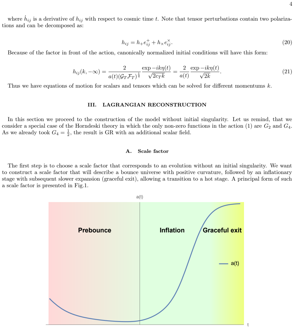
The central object is a four-parameter scale factor built from two sigmoid-weighted power laws, one for the contracting branch and one for inflation, with the compact form $a(t) = \frac{10^{\alpha} t^2 + a_0}{e^{bt}+1} + \frac{10^{\beta}(t-t_b)^n + a_0}{e^{-bt}+1}$. The reconstruction uses the k-essence ansatz $G_2 = g_0(\phi)+g_1(\phi)X$ with $\phi(t)=t$ and $X=1/2$ on shell, which turns the Friedmann equations into two algebraic equations for $g_0$ and $g_1$, avoiding any need to solve differential equations. The key identity is $c_S^2 = F_S/G_S = G_{2X}/(G_{2X}+2X G_{2XX}) = 1$, enforced by dropping the $X^2$ term; together with curvature terms in the background equations, this is what lets the model pass through the bounce with conventional matter and stable perturbations.
What would settle it
For the smallest and largest comoving wavenumbers used in the spectra, compute $k/(aH)$ at the chosen initial integration time; if all values are well below 1, the vacuum initial conditions are being imposed on superhorizon modes. A direct calculation is to integrate each mode starting from the moment $k = aH$ and compare the resulting ($n_s$, $r$) with the paper's claimed contours.
Extended reading notes
Core claim
The paper claims that in the k-essence subclass of generalized scalar-tensor theories, positive spatial curvature allows a nonsingular transition from a contraction phase to inflation with a scalar field whose action is simply $G_2 = g_0(\phi) + g_1(\phi)X$ with $G_4 = 1/2$. The Lagrangian is reconstructed algebraically by fixing $\phi(t)=t$ and $X=1/2$ on shell, and the resulting perturbation functions $F_S$ and $G_S$ stay positive and equal, so the scalar and tensor sound speeds are both unity and no gradient or tachyon instabilities appear. Numerical integration of the perturbation equations with flat-spacetime vacuum initial conditions gives spectral parameters in the range ($n_s$ around 0.96, $r$ around 0.002--0.01 for the examples) that fall within current observational contours. The paper also states that anisotropy growth during contraction is kept subdominant to curvature by assuming an earlier phase that suppressed initial anisotropy, making the bounce curvature-driven rather than anisotropy-driven.
Load-bearing premise
The predicted spectral tilt and tensor-to-scalar ratio depend on setting perturbations to the flat-spacetime vacuum at a fixed early time in the contracting phase, when every finite-wavelength mode is already far outside the horizon, so that vacuum state may not be the physically correct initial condition.
Editorial extensions
If this is right
- A closed universe can pass from contraction to inflation with no exotic matter and no singularity, so the early universe need not begin at a Planck-scale quantum-gravity era.
- The model predicts unit sound speeds for both scalar and tensor perturbations, meaning the primordial spectra keep the standard inflationary shapes and differ from ordinary inflation only through the pre-bounce initial state.
- Because the scale-factor parameters can be varied to produce almost any ($n_s$, $r$) pair, current data cannot single out this model; future tightening of these parameters would be needed to constrain it.
- The finite contraction phase makes anisotropy growth a controlled assumption rather than an automatic property: the bounce remains curvature-driven only if an earlier phase suppressed initial anisotropy.
- The algebraic reconstruction method works for any chosen analytic scale factor, so the same technique can generate new bouncing or emergent-universe models by simply specifying a different $a(t)$.
Reading between the lines
- A natural extension is to evolve perturbations through the full scale factor including the graceful-exit or kination phase and compute the running of the spectral index, which the paper leaves unconstrained.
- The vacuum-initial-condition issue is directly testable: rerun the spectra with initial conditions imposed at horizon crossing $k = aH$ for each mode rather than at one fixed early time; if ($n_s$, $r$) leave the observational contours, the reported agreement is an artifact of the choice of initial time.
- The same reconstruction framework could be adapted to open or flat universes or to different contraction power laws, producing a family of models whose ($n_s$, $r$) maps could be compared with future data.
- A future measurement of the tensor spectral index $n_T$, which the paper does not report, could distinguish this curvature-bounce account from single-field slow-roll inflation even if $n_s$ agrees.
Editorial analysis
A structured set of objections, weighed in public.
Referee Report
Summary. The paper presents a closed-universe k-essence model in which a scale factor describing a curvature bounce followed by inflation is chosen first, and the Lagrangian functions g0(phi) and g1(phi) are then reconstructed algebraically. The authors claim the model is stable, singularity-free, and does not require NEC-violating matter, and they numerically compute the scalar and tensor power spectra, reporting several parameter sets whose (n_s, r) values fall inside the Planck and BICEP/Keck contours (Table I and Fig. 5). The main quantitative claim is therefore that the bounce-to-inflation scenario can match current CMB observations.
Significance. If the reconstruction and the power-spectrum calculation were both sound, the paper would provide a concrete example of a nonsingular bouncing cosmology with conventional scalar matter, unit sound speed, and observables compatible with CMB data. The algebraic reconstruction from the chosen scale factor to g0 and g1 appears coherent, and the stability conditions are checked for selected parameter sets. The paper also explicitly acknowledges several limitations, including the assumed earlier phase that suppresses anisotropy and the absence of a graceful-exit phase in the scale factor used for the spectra. However, these strengths do not compensate for the problems with the vacuum initial conditions and with the tuned, non-predictive nature of the observable fit.
major comments (3)
- [Section IV, Eqs. (14) and (21)] The numerical power spectra are initialized with Minkowski vacuum initial conditions imposed "long before the bounce, when H is small and the vacuum initial conditions can be employed." For the contracting branch of the scale factor (22), a(t) ~ 10^alpha t^2 as t -> -infinity, so H ~ 2/t -> 0^- but a|H| ~ 2*10^alpha |t| -> infinity. Hence for every finite comoving wavenumber k, the ratio k/(a|H|) tends to zero at early times: all modes are superhorizon when the integration starts. A Minkowski vacuum is only an appropriate adiabatic initial state for subhorizon modes, so the initial conditions in (14) and (21) are not justified. The resulting zeta_k and h_k, and therefore P_zeta, P_h, n_s, and r in Table I and Figure 5, are artifacts of an incorrect initial state. The paper does not specify the actual initial time, provide convergence tests, or release code that would allow the calculation to be checked.
- [Section IV, Table I and the paragraph preceding it] The paper states that "by varying the parameters of the scale factor it is possible to achieve almost any values of r and n_s" and then presents six tuned parameter sets lying inside the observational contours. Because the Lagrangian is reconstructed from the scale factor and the parameters are adjusted after knowing the target contours, the agreement in Figure 5 is a fit rather than a falsifiable prediction. To make the observational comparison meaningful, the paper needs either a parameter-independent prediction, a prior or evidence calculation, or predictions for additional observables (e.g., n_T or the running of n_s) that are not used in the fit. As it stands, the claimed agreement with Planck and BICEP/Keck does not provide independent support for the model.
- [Section III E, Eqs. (30) and (31)] The stability claim in the abstract is conditional on an unmodeled earlier phase that suppresses anisotropy before the contracting stage. The paper explicitly says that the mechanism for preparing such an initial state is "beyond the scope of the present work," and the conditions (30)-(31) for suppressing BKL-like modes are not evaluated for the reconstructed Lagrangian. This is an acknowledged input assumption rather than a derived property of the model, and it should be stated as such in the abstract and conclusions rather than folded into the blanket claim of stability.
minor comments (5)
- [Section III A and Appendix A] The text says the graceful exit can be incorporated with an additional sigmoid, but the scale factor (22) used for the power-spectrum calculation contains only the contraction and inflation phases. Please clarify explicitly in Section IV that all numerical results refer to (22), not (A1), and state whether the reconstructed g0 and g1 in Appendix B correspond to (22) or (A1).
- [Figure 2 caption] The caption says "Components of G2 function throughout the whole evolution," but the plotted functions correspond to the two-phase scale factor, not the full evolution including graceful exit. The wording should be corrected to avoid overstating the range of validity.
- [Section III D] The demonstration of "no fine tuning" shows that slightly different initial conditions for a(t) lead to similar trajectories for the chosen reconstructed Lagrangian. This is a stability statement about a particular solution, not an absence of fine-tuning of the action parameters themselves; the wording should be adjusted.
- [Section III C] The phrase "without loss of generality" for setting phi(t)=t and X=1/2 is not explained. A field redefinition can justify fixing the on-shell profile, but the statement as written is too terse and should be expanded.
- [Section IV] The paper should report the numerical integration interval, the number of e-folds before and after the bounce, and the dependence of the results on the choice of initial time. Without these details, the power-spectrum results cannot be reproduced.
Circularity Check
The claimed (n_s, r) agreement is an inverse fit: the scale-factor parameters are selected to land inside the Planck/BICEP contours, so the 'predictions' are forced by the choice of inputs.
-
fitted input called prediction
[Section IV (Observables), after Eq. (37); Table I and Fig. 5]
"It is important to note that by varying the parameters of the scale factor it is possible to achieve almost any values of r and ns, so we find several sets that satisfy both stability conditions (12) and current restrictions [34] for r and ns."
The free parameters of the scale-factor ansatz (22) are varied specifically to make the computed (n_s, r) land inside the allowed contours; those same computed values are then presented in Table I/Fig. 5 as the model's 'observational predictions'. Because the scalar and tensor power spectra are obtained by solving Eqs. (13) and (19) on the background set by these same parameters, the output (n_s, r) is a function of the fitted inputs. With the paper's admission that almost any (n_s, r) can be achieved, the reported agreement with Planck/BICEP is an inverse fit (with parameters tuned to the target observables), not a parameter-free prediction; the table entries are forced by construction.
full rationale
The core construction in Section III is a legitimate reverse-engineering: a nonsingular bouncing scale factor is chosen, and the Lagrangian functions g0 and g1 are solved algebraically from the Friedmann equations, so the background is self-consistent by design. That part is not circular. The circularity is confined to Section IV: the paper fits the scale-factor parameters to the observed n_s and r and then labels the resulting points as predictions. The quoted sentence explicitly concedes that the parameters can be adjusted to reproduce almost any values of n_s and r, which means Table I and Fig. 5 are demonstrations of fit flexibility rather than independent tests of the model. There is no load-bearing self-citation chain: the cited works on gamma-crossing and BKL conditions are external to this paper's derivation, and the reconstruction itself does not rely on the observational constraints. The initial-condition concern about Minkowski vacuum on superhorizon modes is a correctness and physical-reliability issue, not a circularity, so it does not enter the score. Overall, the central quantitative claim reduces to parameter fitting, but the background and stability analysis retain independent content, giving a score of 6 rather than higher.
Assumptions & free parameters
free parameters (6)
- alpha =
-3.57 to -2.22 in Table I
- beta =
-189.52 to -162.56 in Table I
- b =
0.010 to 0.080 in Table I
- n =
50 to 60 in Table I
- t_b =
-1850 to -1495 in Table I
- a0 =
not tabulated
assumptions (5)
- ad hoc to paper The action is restricted to G4 = 1/2 and G2 = g0(phi) + g1(phi)X, with G2XX = 0 to enforce c_s = 1.
- domain assumption The FLRW metric with spatial curvature is assumed throughout contraction, bounce, and inflation.
- ad hoc to paper An earlier phase suppressed the initial anisotropy to very small values before the contracting stage.
- domain assumption Minkowski vacuum initial conditions for perturbations apply at early times in the contracting branch.
- ad hoc to paper The chosen scale factor (22) exactly describes the background evolution, including the bounce and inflation.
Cite this review
Pith. "Pith review of Inflation after Curvature Bounce." pith.science (2026). https://pith.science/paper/ZCSQLAD7
@misc{pith2026241221087,
  author       = {Pith},
  title        = {Pith review of: Inflation after Curvature Bounce},
  year         = {2026},
  howpublished = {\url{https://pith.science/paper/ZCSQLAD7}},
  note         = {Machine review of arXiv:2412.21087}
}
abstract
We present a stable cosmological model of a closed universe in the presence of conventional scalar field. The stability of the model and absence of singularity is ensured by spatial curvature without the need for additional peculiar matter. We reconstruct the Lagrangian and numerically compute observational predictions, including the number of e-folds, the spectral index $n_s$, and the tensor-to-scalar ratio. We present several sets of parameters that satisfy the current observational data.
Figures


Figures from the paper (3 more)


Reference graph
Works this paper leans on
-
[1]
The emergent universe: inflationary cosmology with no singularity,
G. F. R. Ellis and R. Maartens, “The emergent universe: inflationary cosmology with no singularity,” Classical and Quantum Gravity, vol. 21, no. 1, p. 223–232, Nov. 2003. [Online]. Available: http://dx.doi.org/10.1088/0264-9381/21/1/015
-
[2]
Einstein’s 1917 static model of the universe: a centennial review,
C. O’Raifeartaigh, M. O’Keeffe, W. Nahm, and S. Mitton, “Einstein’s 1917 static model of the universe: a centennial review,” Eur. Phys. J. H , vol. 42, no. 3, pp. 431–474, 2017
work page 1917
-
[3]
Although the expression for the scale factor and the corresponding Lagrangian would be considerably extensive, the reconstruction technique remains the same. As our primary focus is on the parameters of the power spectra, we will concentrate solely on the initial two phases. The comprehensive expression of the scale factor is provided in the Appendix A. W...
work page 2000
-
[4]
Big-bang model without singularities,
G. L. Murphy, “Big-bang model without singularities,”Phys. Rev. D , vol. 8, pp. 4231–4233, 1973
work page 1973
-
[5]
On a nonsingular isotropic cosmological model,
A. A. Starobinsky, “On a nonsingular isotropic cosmological model,”Sov. Astron. Lett., vol. 4, p. 82, 1978, [Pis’ma Astron. Zh. 4, 155 (1978)]
work page 1978
-
[6]
The Oscillating Universe: an Alternative to Inflation
R. Durrer and J. Laukenmann, “The oscillating universe: An alternative to inflation,”Class. Quant. Grav. , vol. 13, pp. 1069–1088, 1996. [Online]. Available: https://arxiv.org/pdf/gr-qc/9510041
work page Pith review arXiv 1996
-
[7]
A classical bounce: constraints and consequences
F. T. Falciano, M. Lilley, and P. Peter, “A classical bounce: Constraints and consequences,”Phys. Rev. D , vol. 77, p. 083513, 2008. [Online]. Available: https://arxiv.org/pdf/0802.1196
work page Pith review arXiv 2008
-
[8]
M. NOVELLO and S. BERGLIAFFA, “Bouncing cosmologies,”Physics Reports, vol. 463, no. 4, p. 127–213, Jul. 2008. [Online]. Available: http://dx.doi.org/10.1016/j.physrep.2008.04.006
Show all 38 references
-
[9]
A critical review of classical bouncing cosmologies,
D. Battefeld and P. Peter, “A critical review of classical bouncing cosmologies,”Physics Reports, vol. 571, p. 1–66, Apr
-
[10]
Curvature bounce in general relativity: background and primordial spectrum,
C. Renevey, A. Barrau, K. Martineau, and S. Touati, “Curvature bounce in general relativity: background and primordial spectrum,” Journal of Cosmology and Astroparticle Physics , vol. 2021, no. 01, p. 018–018, Jan. 2021. [Online]. Available: http://dx.doi.org/10.1088/1475-7516...
2021 doi
-
[11]
The emergent universe: an explicit construction,
G. F. R. Ellis, J. Murugan, and C. G. Tsagas, “The emergent universe: an explicit construction,”Classical and Quantum Gravity, vol. 21, no. 1, p. 233–249, Nov. 2003. [Online]. Available: http://dx.doi.org/10.1088/0264-9381/21/1/016
2003 doi
-
[12]
G-bounce,
D. A. Easson, I. Sawicki, and A. Vikman, “G-bounce,” JCAP, vol. 11, p. 021, 2011. [Online]. Available: https://arxiv.org/pdf/1109.1047
2011 arXiv
-
[13]
Galilean genesis: An alternative to inflation,
P. Creminelli, A. Nicolis, and E. Trincherini, “Galilean genesis: An alternative to inflation,”JCAP, vol. 11, p. 021, 2010. [Online]. Available: https://arxiv.org/pdf/1007.0027
2010 arXiv
-
[14]
Towards a nonsingular bouncing cosmology,
Y.-F. Cai, D. A. Easson, and R. Brandenberger, “Towards a nonsingular bouncing cosmology,” Journal of Cosmology and Astroparticle Physics , vol. 2012, no. 08, p. 020–020, Aug. 2012. [Online]. Available: http://dx.doi.org/10.1088/1475-7516/2012/08/020
2012 doi
-
[15]
Bouncing galileon cosmologies,
T. Qiu, J. Evslin, Y.-F. Cai, M. Li, and X. Zhang, “Bouncing galileon cosmologies,”Journal of Cosmology and Astroparticle Physics, vol. 2011, no. 10, p. 036–036, Oct. 2011. [Online]. Available: http://dx.doi.org/10.1088/1475-7516/2011/10/036
2011 doi
-
[16]
Cosmological bounce and Genesis beyond Horndeski,
R. Kolevatov, S. Mironov, N. Sukhov, and V. Volkova, “Cosmological bounce and Genesis beyond Horndeski,”JCAP, vol. 08, p. 038, 2017
2017
-
[17]
Galileon bounce after ekpyrotic contraction,
M. Osipov and V. Rubakov, “Galileon bounce after ekpyrotic contraction,” JCAP, vol. 11, p. 031, 2013. [Online]. Available: https://arxiv.org/pdf/1303.1221
2013 arXiv
-
[18]
Cosmological scenarios with bounce and genesis in horndeski theory and beyond,
V. E. Volkova, S. A. Mironov, and V. A. Rubakov, “Cosmological scenarios with bounce and genesis in horndeski theory and beyond,” Journal of Experimental and Theoretical Physics , vol. 129, no. 4, pp. 553–565, Oct 2019. [Online]. Available: https://doi.org/10.1134/S1063776119100236
2019 doi
-
[19]
A covariant lagrangian for stable nonsingular bounce,
Y. Cai and Y.-S. Piao, “A covariant lagrangian for stable nonsingular bounce,”Journal of High Energy Physics , vol. 2017, no. 9, Sep. 2017. [Online]. Available: http://dx.doi.org/10.1007/JHEP09(2017)027
2017 doi
-
[20]
Stable cosmological solutions in horndeski theory,
S. Mironov and A. Shtennikova, “Stable cosmological solutions in horndeski theory,”Journal of Cosmology and Astroparticle Physics, vol. 2023, no. 06, p. 037, Jun. 2023. [Online]. Available: http://dx.doi.org/10.1088/1475-7516/2023/06/037
2023 doi
-
[21]
Subluminal cosmological bounce beyond horndeski,
S. Mironov, V. Rubakov, and V. Volkova, “Subluminal cosmological bounce beyond horndeski,” Journal of Cosmology and Astroparticle Physics , vol. 2020, no. 05, p. 024–024, May 2020. [Online]. Available: http://dx.doi.org/10.1088/1475-7516/2020/05/024
2020 doi
-
[22]
Generalized multi-Galileons, covariantized new terms, and the no-go theorem for nonsingular cosmologies,
S. Akama and T. Kobayashi, “Generalized multi-Galileons, covariantized new terms, and the no-go theorem for nonsingular cosmologies,” Phys. Rev. D , vol. 95, no. 6, p. 064011, 2017
2017
-
[23]
Second-order scalar-tensor field equations in a four-dimensional space,
G. W. Horndeski, “Second-order scalar-tensor field equations in a four-dimensional space,”International Journal of Theo- retical Physics, vol. 10, no. 6, pp. 363–384, 1974
1974
-
[24]
Non-singular bouncing cosmology with positive spatial curvature and flat scalar potential,
H. Matsui, F. Takahashi, and T. Terada, “Non-singular bouncing cosmology with positive spatial curvature and flat scalar potential,” Physics Letters B , vol. 795, p. 152–159, Aug. 2019. [Online]. Available: http: //dx.doi.org/10.1016/j.physletb.2019.06.013
2019 doi
-
[25]
The null energy condition and its violation,
V. A. Rubakov, “The null energy condition and its violation,”Physics-Uspekhi, vol. 57, no. 2, p. 128–142, Feb. 2014. [Online]. Available: http://dx.doi.org/10.3367/UFNe.0184.201402b.0137
2014
-
[26]
k-essence, superluminal propagation, causality and emergent geometry,
E. Babichev, V. Mukhanov, and A. Vikman, “k-essence, superluminal propagation, causality and emergent geometry,” Journal of High Energy Physics , vol. 2008, no. 02, p. 101–101, Feb. 2008. [Online]. Available: http://dx.doi.org/10.1088/1126-6708/2008/02/101
2008 doi
-
[27]
Transitioning from a bounce to r 2 inflation,
R. Daniel, M. Campbell, C. van de Bruck, and P. Dunsby, “Transitioning from a bounce to r 2 inflation,” Journal of Cosmology and Astroparticle Physics , vol. 2023, no. 06, p. 030, Jun. 2023. [Online]. Available: http://dx.doi.org/10.1088/1475-7516/2023/06/030
2023 doi
-
[28]
Horndeski theory and beyond: a review,
T. Kobayashi, “Horndeski theory and beyond: a review,”Rept. Prog. Phys., vol. 82, no. 8, p. 086901, 2019. 14
2019
-
[29]
From k-essence to generalised Galileons,
C. Deffayet, X. Gao, D. A. Steer, and G. Zahariade, “From k-essence to generalised Galileons,”Phys. Rev. D , vol. 84, p. 064039, 2011
2011
-
[30]
Oscillatory approach to a singular point in the relativistic cosmol- ogy,
V. A. Belinsky, I. M. Khalatnikov, and E. M. Lifshitz, “Oscillatory approach to a singular point in the relativistic cosmol- ogy,” Adv. Phys., vol. 19, pp. 525–573, 1970
1970
-
[31]
Exact scalar field cosmologies,
G. F. R. Ellis and M. S. Madsen, “Exact scalar field cosmologies,”Class. Quant. Grav. , vol. 8, pp. 667–676, 1991
1991
-
[32]
A generalisation of the heckmann–schucking cosmological solution,
I. Khalatnikov and A. Kamenshchik, “A generalisation of the heckmann–schucking cosmological solution,”Physics Letters B, vol. 553, no. 3–4, p. 119–125, Feb. 2003. [Online]. Available: http://dx.doi.org/10.1016/S0370-2693(02)03237-9
2003 doi
-
[33]
Ekpyrotic universe: Colliding branes and the origin of the hot big bang,
J. Khoury, B. A. Ovrut, P. J. Steinhardt, and N. Turok, “Ekpyrotic universe: Colliding branes and the origin of the hot big bang,” Physical Review D, vol. 64, no. 12, Nov. 2001. [Online]. Available: http://dx.doi.org/10.1103/PhysRevD.64.123522
2001 doi
-
[34]
Planck constraints on the tensor-to-scalar ratio,
M. Tristram, A. J. Banday, K. M. Górski, R. Keskitalo, C. R. Lawrence, K. J. Andersen, R. B. Barreiro, J. Borrill, H. K. Eriksen, R. Fernandez-Cobos, T. S. Kisner, E. Martínez-González, B. Partridge, D. Scott, T. L. Svalheim, H. Thommesen, and I. K. Wehus, “Planck constraints ...
-
[35]
Generating cosmological perturbations in non-singular horndeski cosmologies,
Y. Ageeva, P. Petrov, and V. Rubakov, “Generating cosmological perturbations in non-singular horndeski cosmologies,” Journal of High Energy Physics , vol. 2023, no. 1, Jan. 2023. [Online]. Available: http: //dx.doi.org/10.1007/JHEP01(2023)026
2023 doi
-
[38]
Bounce beyond Horndeski with GR asymptotics andγ-crossing,
S. Mironov, V. Rubakov, and V. Volkova, “Bounce beyond Horndeski with GR asymptotics andγ-crossing,” JCAP, vol. 10, p. 050, 2018
2018
-
[2015]
Available: http://dx.doi.org/10.1016/j.physrep.2014.12.004
[Online]. Available: http://dx.doi.org/10.1016/j.physrep.2014.12.004
2014 doi
-
[2021]
Available: http://dx.doi.org/10.1051/0004-6361/202039585
[Online]. Available: http://dx.doi.org/10.1051/0004-6361/202039585
Reviewed August 10, 2026 · model on record in the stance chip above.
Discussion (0). Continue with ORCID to comment.