REVIEW 4 major objections 5 minor 25 references
Methods for traceable scanning magnetometry using single nitrogen vacancy centers in diamond: determining orientation, distance and localization
T0 review · 4 major / 5 minor · reviewed 2026-08-06 · deepseek-v4-flash
Pith's one-line read A scanning NV magnetometer can calibrate its own sensor-sample distance and NV-axis azimuth from stray-field images of simple patterned magnetic films, without a vector magnet.
desk verdict A useful NV calibration protocol with a flawed 'blindness' claim and an overreaching localization section; the d_NV and φ extraction itself is credible and deserves referee time. read the letter →
The pith
A machine-rendered reading of the paper's core claim, the machinery that carries it, and where it could break.
The reading
What carries the argument
The argument is carried by two analytic stray-field models. For a semi-infinite PMA stripe edge, the field components $B_x(x) = \frac{A}{2\pi}\frac{d_{\rm NV}}{(x-x_0)^2+d_{\rm NV}^2}$ and $B_z(x) = -\frac{A}{2\pi}\frac{x-x_0}{(x-x_0)^2+d_{\rm NV}^2}$ make $d_{\rm NV}$ the width-setting parameter of the measured projection $B_{\rm NV}(x) = n_x B_x + n_z B_z + B_0$, so fitting the full profile with $x_0$, $B_0$, and the amplitude $A = \mu_0 M_s$ as free parameters isolates $d_{\rm NV}$. For a PMA disc, the field of a current loop of radius $R$ carrying current $I = \sigma M_s$ yields $B_{\rm NV,\phi}(r,\alpha) = B_0 + \cos\theta\, B_z(r,d_{\rm NV}) + \sin\theta\, B_r(r,d_{\rm NV}) \cos(\alpha-\phi)$, so the angular position of the bright arc along the disc edge encodes $\phi$ while the disc interior brightness fixes the magnetization direction $\sigma$. The inverse-AFM localization rests on a different mechanism: the silicon needle, placed in the optical near field of the NV dipole, quenches the collected fluorescence, producing a dip whose minimum is associated with the NV's lateral position, as supported by FDTD simulations.
What would settle it
Scan the same PMA stripe edge on a planarized sample that has no topographic step and compare the fitted $d_{\rm NV}$ with the value from the 40 nm step sample; if the two differ by more than the 1.95 nm scatter, the constant-height assumption across the etch step is falsified.
Extended reading notes
Core claim
The paper's central claim is that a single NV center in a diamond nanopillar can determine its own two most uncertain geometric parameters, the standoff distance $d_{\rm NV}$ and the azimuthal angle $\phi$ of the NV axis, directly from the magnetic stray fields of simple patterned perpendicularly magnetized films. Fitting line scans across a PMA stripe edge to the analytic dipole-sheet field gives $d_{\rm NV} = 31.5 \pm 1.95$ nm as the mean of ten cuts, and fixing this value in a two-dimensional fit of a PMA disc to a current-loop field model yields $\phi = 98.6^\circ$, $97.3^\circ$, and $95.4^\circ$ on three discs, consistent with the expected $90^\circ$ orientation and reproducible to about $3^\circ$. The same fits also return a stripe magnetization $M_s = 1020 \pm 56$ kA/m, matching SQUID measurements, and a disc value of $M_s = 908 \pm 89$ kA/m. Separately, inverse AFM scans over sharp silicon needles reveal contamination and a fluorescence dip whose position is argued, with FDTD simulation support, to mark the NV's lateral location inside the pillar.
Load-bearing premise
The whole distance calibration rests on the assumption that the NV's height above the sample stays exactly the same while the flat-bottomed diamond pillar crosses the 40 nm etched step at the stripe edge, so the fitted width of the stray-field profile reflects only the NV-sample distance.
Editorial extensions
If this is right
- After calibration, $d_{\rm NV}$ and $\phi$ are known for a probe, so quantitative field reconstruction no longer needs them as free fit parameters, removing a major source of ambiguity in NV magnetometry.
- The calibration can be repeated before each measurement session because it needs only a cleanroom-patterned PMA stripe and disc; this would track drift in standoff caused by contamination or AFM feedback changes.
- The measured $\phi \approx 97.1^\circ$ versus the nominal $90^\circ$ shows that gluing of the probe to the tuning fork introduces a mounting misalignment, so the orientation must be measured per probe rather than assumed from geometry.
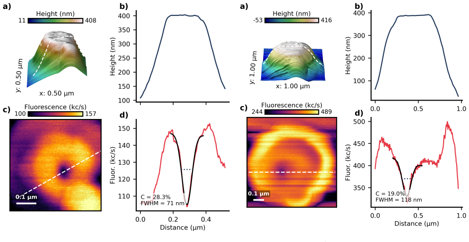
- Inverse AFM topography on sharp silicon needles reveals contamination (here a 19 nm feature on the apex) that would otherwise corrupt the magnetic standoff, and the simultaneously recorded fluorescence dip gives a rough lateral NV localization inside the pillar.
Reading between the lines
- The authors do not automate the routine, but the stripe/disc pair is simple enough that the calibration could be integrated into the standard start-up sequence of any NV microscope, including cryogenic systems where vector magnets are absent.
- Because the FDTD simulation shows a 31.5 nm offset between the fluorescence-dip minimum and the true dipole position, using the dip center as the NV's lateral coordinate would need a position-dependent correction; a full 3D simulation with a realistic pillar apex and the NV's two-dipole emission could quantify that correction.
- The 11% lower $M_s$ extracted from discs than from stripes implies a size-dependent apparent magnetization for small PMA discs; comparing discs of several radii would test whether edge damage from e-beam lithography and ion etching is the cause.
- The $\phi \approx 97^\circ$ result doubles as a probe-mounting diagnostic; collecting this angle for many probes would give a statistical measure of gluing misalignment in commercial sensor assemblies.
Editorial analysis
A structured set of objections, weighed in public.
Referee Report
Summary. The paper proposes a three-step calibration protocol for scanning NV magnetometry. From line scans across PMA stripe edges, the authors extract the NV-to-sample standoff distance d_NV = 31.5 ± 1.95 nm; from two-dimensional maps of PMA discs they extract the NV azimuthal angle φ ≈ 97° (values 98.6°, 97.3°, 95.4°); and from inverse-AFM scans over silicon needles they assess probe contamination and attempt to localize the NV lateral position from a fluorescence dip. The stated advantage is that these parameters are obtained without an external vector magnet, using only simple patterned reference structures.
Significance. If the method is quantitatively reliable, it addresses a real and widely felt need in scanning NV magnetometry: the NV-sample distance and azimuthal orientation are typically unknown or only loosely constrained, and they strongly influence quantitative field reconstruction. The paper includes useful elements: a cross-check of the stripe-derived magnetization against SQUID data, reproducible φ values across three discs, ten statistically analyzed stripe line scans, and publicly archived data. The inverse-AFM part is more exploratory but could be valuable for probe quality control. The main gaps are that the stripe fit is not actually independent of φ, the constancy of d_NV across the topographic step is assumed rather than demonstrated, the fluorescence-dip localization is not quantitatively calibrated, and the reported 'precision' of 3° lacks a proper uncertainty analysis.
major comments (4)
- [Sec. 2.2 and 2.3] The claim that the stripe geometry is 'blind' to the azimuthal angle φ is not correct. Combining Eqs. (4) and (5), the measured projection is B_NV(x) = (A/2π)[sinθ cosφ d/(u²+d²) − cosθ u/(u²+d²)] + B0, so the line shape is a linear combination of Lorentzian and dispersive terms whose relative weight is set by cosφ. The fitting procedure in Sec. 2.3 lists only x0, B0, A and d_NV as free parameters, which implicitly fixes the NV in-plane orientation (likely at the φ = 90° value, for which n_x = 0). For the reported φ ≈ 97° this approximation changes the extremum separation by only about 1.5%, but for a probe with φ = 0° or 180° the extremum separation scales as 2d√(1 + tan²θ cos²φ), which would overestimate d_NV by roughly 73%. Since d_NV is subsequently used as a fixed input to the disc fits, this dependence is load-bearing. The authors should either fit independent Lorentzian and dispersive amplitudes (which would make d_NV identifiable without knowing φ) or explicitly state the assumed φ and propagate its uncertainty into d_NV and the later disc analysis.
- [Sec. 2.5 and Fig. 5] The extraction of d_NV from stripe edge scans assumes that the NV-to-sample standoff remains constant while the flat-bottomed pillar crosses the 40 nm etch step. The argument in Sec. 2.5 — that the apex descends onto the substrate only after completely passing the edge — is plausible but not verified. A small pillar tilt, an off-center NV, or AFM setpoint drift could change the effective contact point during the crossing, which would bias every fitted d_NV and propagate into the disc-derived φ and M_s. The agreement of the fitted M_s with SQUID is encouraging, but it does not by itself rule out a correlated error in d_NV and A. I recommend a control experiment, for example line scans on structures with different step heights or with varied AFM setpoints, to bound this systematic error.
- [Sec. 3 and Fig. 11] The inverse-AFM localization claim is not quantitatively established. The FDTD simulation shows a 31.5 nm offset between the fluorescence-dip minimum and the dipole position, and the simulated contrast and FWHM do not reproduce the measured values, as the text acknowledges. Nevertheless, the paper interprets experimental dip positions as NV lateral positions (for instance, the 80 nm off-center shift for the MX+ probe). Without a validated correction for the offset or an uncertainty estimate, the localization is at best qualitative. The authors should either validate the mapping by an independent method, apply a theoretically justified correction with an uncertainty, or explicitly restrict the claim to qualitative localization.
- [Sec. 3 and Fig. 6] The stated 'precision of 3°' for the azimuthal angle is based on only three discs (φ = 98.6°, 97.3°, 95.4°) and no per-fit uncertainties are reported. The 3° value is the range of the three measurements, not a standard deviation or confidence interval. In addition, the sensitivity of the fitted φ to the fixed value d_NV = 31.5 nm is not discussed. To support the word 'traceable' in the title and abstract, the authors should provide fit uncertainties for each disc and propagate the d_NV uncertainty into φ.
minor comments (5)
- [Sec. 3, Fig. 8] In the description of Fig. 8, 'we this fluorescence dip to the position' should read 'we attribute this fluorescence dip to the position'.
- [Fig. 11 caption] The caption contains 'obtained by diving the collected farfield emission'; 'diving' should be 'dividing'.
- [Sec. 2.5] The text contains 'arising from the the Pt/Co interface'; the duplicated article should be removed.
- [Eqs. (6)–(7)] The quantity P is used in Eq. (6) but defined only in the broken line following Eq. (7); for readability, define P and q together with the other symbols before Eq. (6).
- [Fig. 5(b)] The 1.95 nm standard deviation is described as the spread across ten line scans; please clarify whether this is the standard deviation of the population or of the mean, and give the combined uncertainty that includes the per-fit covariance errors.
Circularity Check
No significant circularity: d_NV and phi are outputs of least-squares fits to measured stray-field maps, with stripe M_s cross-checked against independent SQUID data; self-citations are background only.
full rationale
The claimed derivations are self-contained inversions of measured data rather than re-statements of inputs. B_NV is obtained from ODMR Zeeman splittings (Eq. 3); the stripe and disc stray fields are modeled from standard magnetostatics (Eqs. 4-7); and d_NV, phi, A, x0, B0, R, and I are free parameters of least-squares fits to independently measured line scans and maps. The stripe fit returns M_s = 1020 +/- 56 kA/m and is compared with the as-grown film SQUID value of 1116 kA/m, so the fit is anchored to an external benchmark rather than to the target d_NV. The disc fit subsequently extracts phi with d_NV fixed, and the phi values (98.6, 97.3, 95.4 deg) are cross-checked against the crystallographic expectation of 90 deg. The inverse-AFM fluorescence dip is interpreted via FDTD simulation, not via a parameter fitted to the same data. Self-citations ([4], [12]) are used only as background for transverse ODMR contrast and fluorescence-waveguide coupling; neither is load-bearing, and no uniqueness theorem is invoked. The paper's own admission that the FDTD model does not quantitatively match measured dip contrast and FWHM (Section 3, Figure 11) is a validation gap for the localization claim, not a circular reduction. A separate, non-circular correctness risk is the possible phi-dependence of the stripe line shape despite the statement that the stripe geometry is blind to phi; this concerns identifiability and bias, not equivalence of outputs to inputs.
Assumptions & free parameters
free parameters (10)
- d_NV (NV-sample standoff) =
31.5 ± 1.95 nm (mean of ten line-scan fits)
- A = μ0 M_s t (stripe amplitude) =
M_s = 1020 ± 56 kA/m from fits
- B0 (uniform bias field) =
1.03 mT (disc example)
- x0 (stripe magnetic edge position) =
not quoted
- phi (NV azimuthal angle) =
98.6, 97.3, 95.4 degrees (three discs)
- R (disc radius) =
2.43 μm (one disc)
- disc center (x0,y0) =
not quoted
- I = sigma M_s t (disc loop current) =
M_s = 997 kA/m (one disc); 908 ± 89 kA/m (three discs)
- Gaussian dip parameters (center, FWHM, contrast) =
FWHM 71-175 nm; contrast 14.5-28.3 percent
- d_Si-D (needle-pillar distance in FDTD) =
1-20 nm; 20 nm corresponds to d_NV = 30 nm
assumptions (7)
- domain assumption PMA stripe stray field is the surface dipole field of a semi-infinite thin film with uniform magnetization; film thickness t is negligible compared to d_NV.
- domain assumption PMA disc stray field equals that of a circular current loop of radius R carrying current I = sigma*M_s*t.
- domain assumption The NV polar angle is theta = 54.7 degrees for a (100) diamond nanopillar, and phi is one of four <111> in-plane projections separated by 90 degrees.
- domain assumption The flat-bottomed pillar maintains constant d_NV across the 40 nm topographic etch step.
- domain assumption The bias field B0 is uniform over the scan area, and comparing disc interior vs far background fixes the magnetization sign sigma.
- ad hoc to paper A single tilted electric dipole in a simplified 2D FDTD model captures the fluorescence dip well enough to localize the NV laterally.
- standard math Zeeman splitting Delta f = 2 gamma_NV B_NV is the correct relation between ODMR frequency splitting and the field projection.
Cite this review
Pith. "Pith review of Methods for traceable scanning magnetometry using single nitrogen vacancy centers in diamond: determining orientation, distance and localization." pith.science (2026). https://pith.science/paper/ZIZOKJSR
@misc{pith2026260804632,
  author       = {Pith},
  title        = {Pith review of: Methods for traceable scanning magnetometry using single nitrogen vacancy centers in diamond: determining orientation, distance and localization},
  year         = {2026},
  howpublished = {\url{https://pith.science/paper/ZIZOKJSR}},
  note         = {Machine review of arXiv:2608.04632}
}
read the original abstract
Individual, scannable nitrogen vacancy (NV) centers in single crystal diamond nanostructures enable nanoscale, quantitative imaging of magnetic stray fields. Nevertheless, important parameters like distance between the NV center and the sample and the orientation of the NV high symmetry axis are often not known precisely and enter data evaluation as free fitting parameters. We here use scanning NV imaging on micro-patterned, perpendicularly magnetized stripes and discs. From these measurements, we directly infer NV - sample distance d_NV and the NV's azimuthal orientation without the need for an external vector magnet control. We determine d_NV = 31.5 nm, while we infer the azimuthal orientation with a precision of 3{\deg}. We additionally employ commercially available silicon needles to image the apex topography of our diamond nanostructures to detect surface contamination. Simultaneously, monitoring NV fluorescence as a function of the needle's position allows us to estimate the lateral placement of the NV inside the diamond nanostructure.
Figures


Figures from the paper (7 more)



Reference graph
Works this paper leans on
-
[1]
I. Gross, W. Akhtar, V. Garcia, L. J. Mart ´ ınez, S. Chouaieb, K. Garcia, C. Carr´ et´ ero, A. Barth´ el´ emy, P. Appel, P. Maletinsky, J.- V. Kim, J.-Y. Chauleau, N. Jaouen, M. Viret, M. Bibes, S. Fusil, and V. Jacques. Real-space 14 imaging of non-collinear antiferromagnetic or- der with a single-spin magnetometer.Nature, 549(7671):252–256, September 2017
work page 2017
-
[2]
J.-P. Tetienne, T. Hingant, L. J. Mart ´ ınez, S. Rohart, A. Thiaville, L. Herrera Diez, K. Gar- cia, J.-P. Adam, J.-V. Kim, J.-F. Roch, I. M. Miron, G. Gaudin, L. Vila, B. Ocker, D. Rav- elosona, and V. Jacques. The nature of domain walls in ultrathin ferromagnets revealed by scan- ning nanomagnetometry.Nature Communica- tions, 6(1):6733, April 2015
work page 2015
- [3]
-
[4]
Ephraim Spindler, Vinayak Shantaram Bhat, Elke Neu, Mathias Weiler, and M. Benjamin Jungfleisch. Nanoscale dipolar fields in artificial spin ice probed by scanning NV magnetometry,
-
[5]
Imaging non-collinear antifer- romagnetic textures via single spin relaxometry
Aurore Finco, Angela Haykal, Rana Tanos, Florentin Fabre, Saddem Chouaieb, Waseem Akhtar, Isabelle Robert-Philip, William Legrand, Fernando Ajejas, Karim Bouzehouane, Nicolas Reyren, Thibaut Devolder, Jean-Paul Adam, Joo-Von Kim, Vincent Cros, and Vincent Jacques. Imaging non-collinear antifer- romagnetic textures via single spin relaxometry. Nature Commu...
work page 2021
-
[6]
M. Pelliccione, B. A. Myers, L. M. A. Pascal, A. Das, and A. C. Bleszynski Jayich. Two- dimensional nanoscale imaging of gadolinium spins via scanning probe relaxometry with a sin- gle spin in diamond.Physical Review Applied, 2(5):054014, November 2014
work page 2014
-
[7]
Brecht G. Simon, Samer Kurdi, Joris J. Carmiggelt, Michael Borst, Allard J. Katan, and Toeno van der Sar. Filtering and imaging of frequency-degenerate spin waves using nanopo- sitioning of a single-spin sensor.Nano Letters, 22(22):9198–9204, October 2022
work page 2022
-
[8]
P. Maletinsky, S. Hong, M. S. Grinolds, B. Haus- mann, M. D. Lukin, R. L. Walsworth, M. Lon- car, and A. Yacoby. A robust scanning dia- mond sensor for nanoscale imaging with single nitrogen-vacancy centres.Nature Nanotechnol- ogy, 7(5):320–324, April 2012
work page 2012
Show all 25 references
-
[9]
D. M. Toyli, C. D. Weis, G. D. Fuchs, T. Schenkel, and D. D. Awschalom. Chip-scale nanofabrication of single spins and spin arrays in diamond.Nano Letters, 10(8):3168–3172, 2010
2010
-
[10]
Palm, William Huxter, Konstantin Herb, John M
Zhewen Xu, Marius L. Palm, William Huxter, Konstantin Herb, John M. Abendroth, Karim Bouzehouane, Olivier Boulle, Mihai S. Gabor, Joseba Urrestarazu Larranaga, Andrea Morales, Jan Rhensius, Gabriel Puebla-Hellmann, and Christian L. Degen. Minimizing sensor-sample distances in ...
2025
-
[11]
Thiel, D
L. Thiel, D. Rohner, M. Ganzhorn, P. Appel, E. Neu, B. M¨ uller, R. Kleiner, D. Koelle, and P. Maletinsky. Quantitative nanoscale vortex imaging using a cryogenic quantum magnetome- ter.Nature Nanotechnology, 11(8):677–681, May 2016
2016
-
[12]
Optimized single-crystal diamond scan- ning probes for high sensitivity magnetometry
Philipp Fuchs, Michel Challier, and Elke Neu. Optimized single-crystal diamond scan- ning probes for high sensitivity magnetometry. New Journal of Physics, 20(12):125001, Decem- ber 2018
2018
-
[13]
PhD thesis, University of Cam- bridge, 2023
Michael Hoegen.Probing Two-Dimensional Magnetic Phenomena with Diamond Quantum Microscopy. PhD thesis, University of Cam- bridge, 2023. Apollo – University of Cambridge Repository
2023
-
[14]
Hingant, J.-P
T. Hingant, J.-P. Tetienne, L. J. Mart ´ ınez, K. Garcia, D. Ravelosona, J.-F. Roch, and V. Jacques. Measuring the magnetic moment density in patterned ultrathin ferromagnets with submicrometer resolution.Physical Review Ap- plied, 4(1):014003, 2015. 15
2015
-
[15]
J. D. Jackson.Classical Electrodynamics. Wiley, 3 edition, 1998
1998
-
[16]
J. C. Simpson, J. E. Lane, C. D. Immer, and R. C. Youngquist. Simple analytic expres- sions for the magnetic field of a circular cur- rent loop. Technical Report NASA/TM–2001– 211239, NASA, 2001
2001
-
[17]
Lumerical fdtd: 3d electro- magnetic simulator
Ansys Lumerical. Lumerical fdtd: 3d electro- magnetic simulator. Ansys Lumerical, 2026. Ver- sion 2026 R1
2026
-
[18]
H. R. Phillip and E. A. Taft. Kramers-kronig analysis of reflectance data for diamond.Physi- cal Review, 136(5A):A1445–A1448, 1964
1964
-
[19]
Palik, editor.Handbook of Optical Constants of Solids
Edward D. Palik, editor.Handbook of Optical Constants of Solids. Academic Press, Boston, 1985
1985
-
[20]
D. T. Pierce and W. E. Spicer. Electronic struc- ture of amorphous si from photoemission and op- tical studies.Physical Review B, 5(8):3017–3029, 1972
1972
-
[21]
QuantileverMX product brochure, 2021
Qnami AG. QuantileverMX product brochure, 2021
2021
-
[22]
Dong-Soo Han, Kyujoon Lee, Jan-Philipp Hanke, Yuriy Mokrousov, Kyoung-Whan Kim, Woosuk Yoo, Youri Hees, Tae-Wan Kim, Reinoud Lavrijsen, Chun-Yeol You, Henk J. M. Swagten, Myung-Hwa Jung, and Mathias Kl¨ aui. Long-range chiral exchange interaction in syn- thetic antiferromagnet...
2019
-
[23]
Fabian Kammerbauer, Won-Young Choi, Frank Freimuth, Kyujoon Lee, Robert Fr¨ omter, Dong- Soo Han, Reinoud Lavrijsen, Henk J. M. Swagten, Yuriy Mokrousov, and Mathias Kl¨ aui. Controlling the interlayer dzyaloshinskii–moriya interaction by electrical currents.Nano Letters, 23(1...
2023
-
[24]
Photonic nano-structures on (111)-oriented dia- mond.Applied Physics Letters, 104(15):153108, April 2014
Elke Neu, Patrick Appel, Marc Ganzhorn, Javier Miguel-S´ anchez, Margarita Lesik, Vian- ney Mille, Vincent Jacques, Alexandre Tal- laire, Jocelyn Achard, and Patrick Maletinsky. Photonic nano-structures on (111)-oriented dia- mond.Applied Physics Letters, 104(15):153108, April 2014
2014
-
[25]
Mayer Alegre, Charles Santori, Gilberto Medeiros-Ribeiro, and Raymond G
Thiago P. Mayer Alegre, Charles Santori, Gilberto Medeiros-Ribeiro, and Raymond G. Beausoleil. Polarization-selective excitation of nitrogen vacancy centers in diamond.Physical Review B, 76(16):165205, October 2007. 16
2007
Reviewed August 6, 2026 · model on record in the stance chip above.
Discussion (0). Continue with ORCID to comment.