REVIEW 3 major objections 3 minor 1 cited by
SNAP: Sequential Non-Ancestor Pruning for Targeted Causal Effect Estimation With an Unknown Graph
T0 review · 3 major / 3 minor · reviewed 2026-08-08 · deepseek-v4-flash
Pith's one-line read The full causal graph is unnecessary for targeted effect estimation: a sequential pruning algorithm that keeps only possible ancestors of the targets recovers exactly the relevant CPDAG.
desk verdict Useful targeted causal discovery method, but the k=1 soundness proof has a concrete lemma-application gap that needs fixing before the prefiltering claims are credible. read the letter →
The pith
A machine-rendered reading of the paper's core claim, the machinery that carries it, and where it could break.
The reading
What carries the argument
The central object is the set of possible ancestors of the targets. In a CPDAG $G$, a node $X$ is a possible ancestor of $Y$ when a possibly directed path connects them — a path made of undirected edges and edges pointing toward $Y$ — which is equivalent to $X$ being an ancestor of $Y$ in at least one DAG of the Markov equivalence class. The load-bearing identity is Lemma 3.1: a possibly ancestral set $V^*$ that contains $\mathrm{PossAn}(T)$ induces the same CPDAG as the full graph restricted to $V^*$, so discovery can be confined to $V^*$ without losing any informative adjustment set. The algorithm's mechanism is a loop that runs a PC-style skeleton search with conditioning sets of size $i$, orients v-structures (using PC rules for $i \in \{0,1\}$ and RFCI-style rules with extra dependency checks for $i \geq 2$, because low-order tests can create conflicting v-structures even when the underlying edge is real), and then removes every node with no possibly directed path to a target. The safety of the cheap PC-style orientation at order 1 rests on a d-separation lemma about treks (Lemma B.3), applied repeatedly.
What would settle it
Enumerate all labeled DAGs on four nodes and check Lemma B.3 directly: any quadruple $(W, X, Y, Z)$ in which $X$ and $Y$ are d-connected given the empty set, $X \perp\!\!\!\perp_d Y \mid Z$ and $Z \perp\!\!\!\perp_d Y \mid W$ both hold, but $X \perp\!\!\!\perp_d Y \mid W$ fails, is a counterexample that collapses the order-1 soundness proof. A complementary end-to-end check is to run SNAP(1) with oracle d-separation tests over all DAGs up to six nodes and all possible target sets, recording the first graph in which a true possible ancestor of a target is pruned.
Extended reading notes
Core claim
The paper establishes that definite non-ancestors of the targets are unnecessary for learning causal relations among the targets and for identifying efficient adjustment sets. Theorem 3.1 states that, given oracle conditional independence tests, every iteration of SNAP(k) retains all possible ancestors of the targets and leaves a possibly ancestral set, one that contains all of its own possible ancestors. Lemma 3.1 then guarantees that any possibly ancestral set containing the targets' possible ancestors yields the same canonical, parental, ancestor, and asymptotically optimal adjustment sets as the full CPDAG. Theorem 3.2 completes the picture: SNAP(∞), the standalone variant, returns exactly $\hat{G} = G|_{\mathrm{PossAn}(T)}$, the induced subgraph of the full CPDAG over the possible ancestors of the target set, and is sound and complete over that subgraph. The upshot is that recovering the complete CPDAG over all variables is not required for targeted causal effect estimation; the relevant subgraph suffices, and pruning can happen during discovery rather than after it.
Load-bearing premise
The soundness guarantee assumes oracle conditional-independence tests, and within that idealization the fragile step is Lemma B.3, a d-separation implication about treks that lets SNAP orient v-structures cheaply at order 1; if that implication fails in any configuration, a true possible ancestor of the targets could be mislabeled as a definite non-ancestor and pruned.
Editorial extensions
If this is right
- Stopping SNAP(k) at any order and running a sound-and-complete discovery algorithm on the survivors returns the induced subgraph of the full CPDAG restricted to those variables, so all informative adjustment sets for the target effects are preserved (Corollary 3.1).
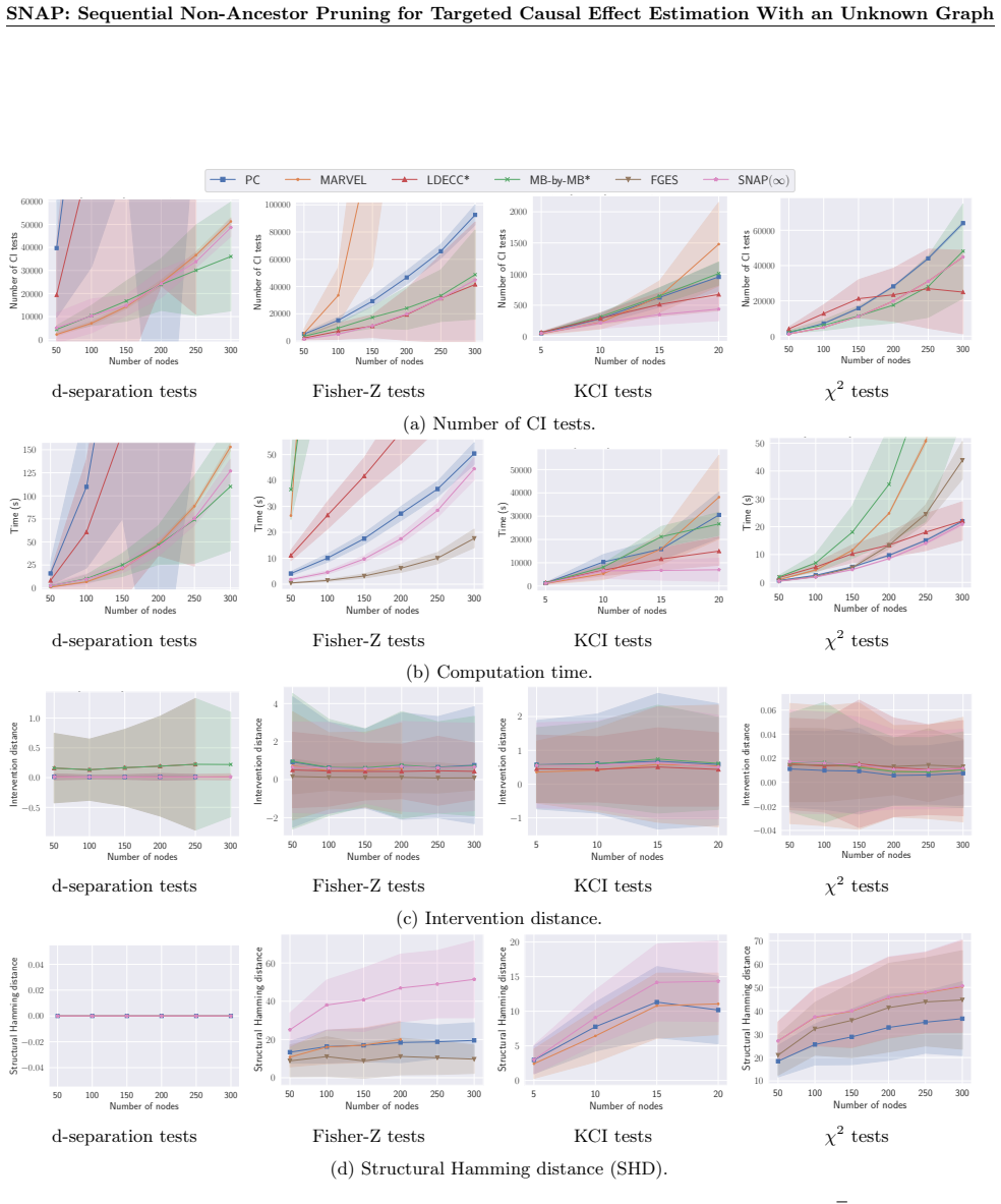
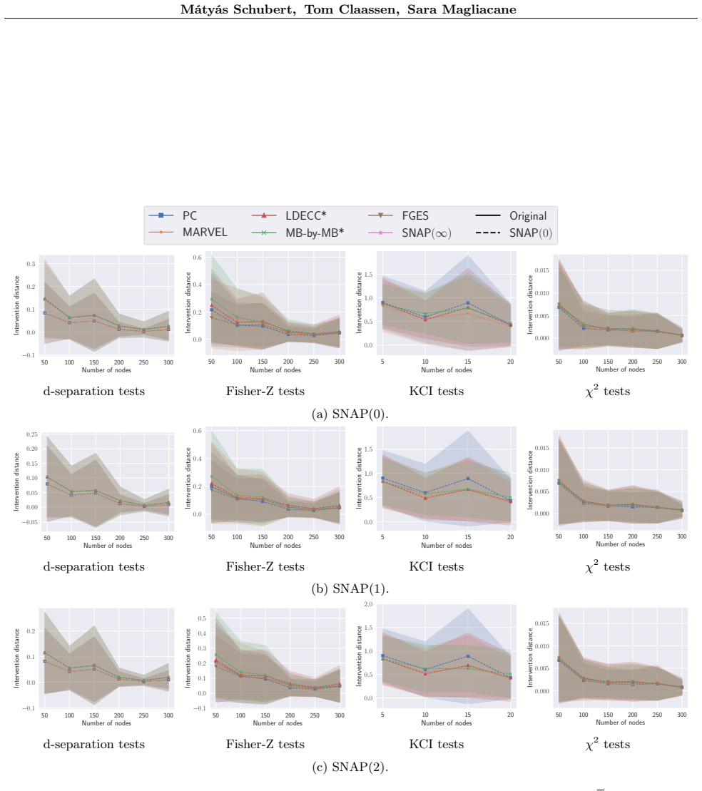
- Even SNAP(0), which prunes purely on marginal-independence information, already cuts independence tests and runtime by large factors as a prefilter in the reported experiments, and it consistently improved PC, MARVEL, and MB-by-MB* across settings.
- SNAP(∞) as a standalone method recovers exactly the induced CPDAG over $\mathrm{PossAn}(T)$, and its worst-case complexity of $O(|V|^{d_{\max}+2} + |V|^4)$ matches PC's $O(|V|^{d_{\max}+2})$ for graphs with maximum degree at least 2.
- SNAP's cost is nearly constant as the number of targets grows, because all targets are handled jointly, whereas local methods that process targets one at a time degrade substantially with more targets.
- Because SNAP concentrates its independence tests at low orders, it avoids high-order conditional-independence tests, which are statistically weaker for kernel-based and $\chi^2$ tests.
Reading between the lines
- My inference: the 'possible ancestors are all you need' principle should carry over to causally insufficient settings, where the analogous object is the set of nodes possibly ancestral to the targets in a partial ancestral graph; the paper names this as future work, and nothing in Lemma 3.1 depends essentially on causal sufficiency.
- My inference: SNAP's prefiltering is agnostic to the downstream method, so it should combine equally well with score-based discovery, where the reduced variable set also shrinks the search space over DAGs.
- My inference: the paper's own finite-sample diagnostics (App. D.9) find more missing than extra edges and attribute them to pruning the wrong nodes, which suggests that a confidence-aware pruning rule — keeping nodes whose possible-ancestor status is borderline — could close the gap between the oracle soundness guarantee and finite-sample behaviour; the paper does not pursue this.
- My inference: Lemma B.3 is a purely discrete statement about d-separation, so exhaustive enumeration over all four-node DAGs would certify or refute it outright, a check that costs almost nothing and would settle the most fragile step of the proof.
Editorial analysis
A structured set of objections, weighed in public.
Referee Report
Summary. The paper addresses targeted causal effect estimation with an unknown graph: rather than learning a full CPDAG over all variables, it proposes to learn only a subgraph over a possibly ancestral superset of the possible ancestors of a small target set T. The central claim is that definite non-ancestors of T are unnecessary both for identifying causal relations among targets and for finding valid and efficient adjustment sets. The proposed SNAP(k) algorithm interleaves a PC-style skeleton search with orientation of v-structures and iterative pruning of nodes that have no possibly directed path to T; SNAP(∞) adds Meek rule completion and is claimed to return exactly the induced CPDAG over PossAn(T). The paper gives oracle soundness/completeness theorems (Theorems 3.1 and 3.2), a worst-case complexity analysis, and extensive experiments on synthetic data and two real benchmark networks.
Significance. If the oracle claims are correct, the paper makes a useful step: it formalizes a targeted discovery task and shows that only possible ancestors of the target set need to be retained, building on known ancestral-set preservation results of Lauritzen and Guo et al. The paper is strong on framing, has extensive experiments with several CI test families, reports both computational and effect-estimation metrics, and releases code. No fitted constants or circularity in the main theorems was found. However, the k=1 soundness proof contains a concrete gap in the appendix, and Theorem 3.2 and the prefiltering Corollary 3.1 rely on that k=1 case. Because SNAP(1) and SNAP(∞) are central to the paper's practical claims, this gap is load-bearing and prevents accepting the paper in its current form.
major comments (3)
- [Appendix B, Lemma B.4] The proof of the k=1 case applies Lemma B.3 with a substitution that does not fit the lemma's statement. Lemma B.3 states: if X and Y are d-connected given the empty set, X⊥d Y | Z, and Z⊥d Y | W, then X⊥d Y | W. In Lemma B.4, to conclude X⊥d Z | {V}, the proof requires the third antecedent to be W⊥d Z | {V}. Instead, the displayed implication uses X⊥d W | {V}. Thus the claimed derivation is not an instance of Lemma B.3, and the same mismatch recurs in the 'two successive applications' argument later in the same proof. As written, the k=1 case of Theorem 3.1 is not established, and since Theorem 3.2 and Corollary 3.1 depend on Theorem 3.1, the central soundness claim that SNAP(1) prunes only definite non-ancestors is not backed by the supplied proof.
- [Appendix B, Lemma B.4 and Theorem 3.1] The repeated-application argument in Lemma B.4 is an inductive chain over non-adjacent nodes, but each step invokes the same unmatched form of Lemma B.3. Even if the intended implication 'X⊥d Z|{W}, X⊥d W|{V}, X not⊥d Z implies X⊥d Z|{V}' were true, it is not proved in the paper; the proof as written is therefore incomplete for every iteration in the chain, not just the first step. The authors should either state and prove the correct auxiliary lemma, or modify the algorithm so that the RFCI dependency checks are also used at iteration k=1.
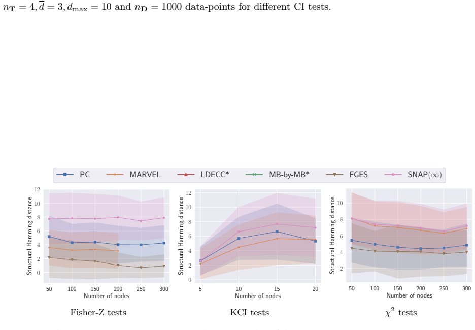
- [Appendix D.9] The paper itself reports that, in finite samples, missing edges in SNAP(∞)'s output arise not from type II CI-test errors but from pruning the wrong nodes. This is an honest limitation statement, but it should be weighed explicitly against the abstract's unqualified claim that pruning is done without compromising estimation quality. The oracle theorems are not contradicted by this finite-sample behavior, but the main text should state that the 'prunes only definite non-ancestors' guarantee holds only with oracle CI tests, and that finite-sample SNAP can remove true possible ancestors, with the experimental support for the no-compromise claim resting on intervention distance rather than structural fidelity.
minor comments (3)
- [Theorem 3.1] The theorem says a set is possibly ancestral, 'i.e., PossAn_G(\hat V_i) ⊆ \hat V_{i+1}'. The displayed condition is stronger than the definition of \hat V_{i+1} being possibly ancestral, which should be PossAn_G(\hat V_{i+1}) ⊆ \hat V_{i+1}. The proof establishes the stronger statement, but the wording is imprecise.
- [Section 3.2 / Section 6] The conclusion refers to 'SNAP(1), a stand-alone sound and complete discovery algorithm', while the rest of the paper defines SNAP(∞) as the sound and complete stand-alone algorithm. This appears to be a typo and should be corrected.
- [Appendix B.3] In the proof of Corollary 3.1, the sentence 'from the application of Theorem 3.1, that shows that a possibly ancestral set...' should presumably refer to Lemma 3.1, not Theorem 3.1.
Circularity Check
No significant circularity: the soundness theorems follow from d-separation arguments and externally cited lemmas, with no fitted parameters, self-citation chain, or definitional reduction.
full rationale
The paper's central claim is that definite non-ancestors of target variables are unnecessary for targeted causal effect estimation, and that SNAP(k) prunes only such nodes. This claim is supported by Theorem 3.1, whose proof rests on Lemma B.2 and Lemma B.4, both of which are d-separation arguments about the ground-truth DAG, and on Lemma B.3, a standalone graphical claim. The key graph-restriction result, Lemma 3.1, is imported from Lauritzen (1996) and Guo et al. (2023), which are external sources, not self-citations. The algorithm contains no fitted constants and no parameter is calibrated to the evaluation data; the experiments are benchmarked against synthetic ground-truth graphs and real networks, so the reported reductions in CI tests and runtime are not forced by construction. The only adoption of prior work is the use of RFCI orientation rules from Colombo et al. (2012), which is an external, independently established algorithm used as a building block, not an unverified premise that is doing the load-bearing work. The skeptical concern in the review about Lemma B.3 possibly being applied with mismatched conditioning sets is a potential correctness gap in the k=1 proof, not a circularity: it would make a theorem unproven if valid, but it does not make the theorem's conclusion an input to its own proof. There are no self-citations of the present authors at all, and no uniqueness theorem is invoked from the authors' prior work. Overall, the derivation chain is self-contained relative to standard external results, and no step was found in which a prediction reduces to its own inputs by definition or by fitting.
Assumptions & free parameters
assumptions (4)
- domain assumption Causal sufficiency: no unobserved confounders or selection bias
- domain assumption Markov and faithfulness of the observational distribution to the causal DAG
- domain assumption Oracle conditional independence tests for the theoretical guarantees
- standard math Known results on ancestral sets and CPDAG restriction (Lauritzen Proposition 3.22 and Guo et al. Lemma D.1)
Cite this review
Pith. "Pith review of SNAP: Sequential Non-Ancestor Pruning for Targeted Causal Effect Estimation With an Unknown Graph." pith.science (2026). https://pith.science/paper/ZJJFX3P3
@misc{pith2026250207857,
  author       = {Pith},
  title        = {Pith review of: SNAP: Sequential Non-Ancestor Pruning for Targeted Causal Effect Estimation With an Unknown Graph},
  year         = {2026},
  howpublished = {\url{https://pith.science/paper/ZJJFX3P3}},
  note         = {Machine review of arXiv:2502.07857}
}
read the original abstract
Causal discovery can be computationally demanding for large numbers of variables. If we only wish to estimate the causal effects on a small subset of target variables, we might not need to learn the causal graph for all variables, but only a small subgraph that includes the targets and their adjustment sets. In this paper, we focus on identifying causal effects between target variables in a computationally and statistically efficient way. This task combines causal discovery and effect estimation, aligning the discovery objective with the effects to be estimated. We show that definite non-ancestors of the targets are unnecessary to learn causal relations between the targets and to identify efficient adjustments sets. We sequentially identify and prune these definite non-ancestors with our Sequential Non-Ancestor Pruning (SNAP) framework, which can be used either as a preprocessing step to standard causal discovery methods, or as a standalone sound and complete causal discovery algorithm. Our results on synthetic and real data show that both approaches substantially reduce the number of independence tests and the computation time without compromising the quality of causal effect estimations.
Figures


Figures from the paper (35 more)







Forward citations
Cited by 1 Pith paper
-
Knowledge-Informed Local Causal Discovery of Optimal Adjustment Sets
Integrating required edge constraints into local structure learning via Meek propagation yields knowledge-constrained MPDAGs that recover optimal adjustment sets not identifiable from observational data alone.
Reference graph
Works this paper leans on
-
[1]
Subset verification and search algorithms for causal dags
Davin Choo and Kirankumar Shiragur. Subset verification and search algorithms for causal dags. In International Conference on Artificial Intelligence and Statistics, pages 4409--4442. PMLR, 2023
work page 2023
-
[2]
Learning high-dimensional directed acyclic graphs with latent and selection variables
Diego Colombo, Marloes H Maathuis, Markus Kalisch, and Thomas S Richardson. Learning high-dimensional directed acyclic graphs with latent and selection variables. The Annals of Statistics, pages 294--321, 2012
work page 2012
-
[3]
The igraph software package for complex network research
Gabor Csardi and Tamas Nepusz. The igraph software package for complex network research. InterJournal, Complex Systems: 0 1695, 2006
work page 2006
-
[4]
Local causal discovery with linear non-gaussian cyclic models
Haoyue Dai, Ignavier Ng, Yujia Zheng, Zhengqing Gao, and Kun Zhang. Local causal discovery with linear non-gaussian cyclic models. In International Conference on Artificial Intelligence and Statistics, pages 154--162. PMLR, 2024
work page 2024
-
[5]
Local causal discovery of direct causes and effects
Tian Gao and Qiang Ji. Local causal discovery of direct causes and effects. Advances in Neural Information Processing Systems, 28, 2015
work page 2015
-
[6]
Review of causal discovery methods based on graphical models
Clark Glymour, Kun Zhang, and Peter Spirtes. Review of causal discovery methods based on graphical models. Frontiers in Genetics, 10, 2019. ISSN 1664-8021. doi:10.3389/fgene.2019.00524
arXiv 2019
-
[7]
Valid inference after causal discovery
Paula Gradu, Tijana Zrnic, Yixin Wang, and Michael Jordan. Valid inference after causal discovery. In NeurIPS 2022 Workshop on Causality for Real-world Impact, 2022
work page 2022
-
[8]
Variable elimination, graph reduction and the efficient g-formula
F Richard Guo, Emilija Perkovi \'c , and Andrea Rotnitzky. Variable elimination, graph reduction and the efficient g-formula. Biometrika, 110 0 (3): 0 739--761, 2023
work page 2023
Show all 49 references
-
[9]
Local causal discovery for estimating causal effects
Shantanu Gupta, David Childers, and Zachary Chase Lipton. Local causal discovery for estimating causal effects. In Conference on Causal Learning and Reasoning, pages 408--447. PMLR, 2023
2023
-
[10]
Exploring network structure, dynamics, and function using networkx
Aric Hagberg, Pieter Swart, and Daniel S Chult. Exploring network structure, dynamics, and function using networkx. Technical report, Los Alamos National Lab.(LANL), Los Alamos, NM (United States), 2008
2008
-
[11]
Learning bayesian networks: The combination of knowledge and statistical data
David Heckerman, Dan Geiger, and David M Chickering. Learning bayesian networks: The combination of knowledge and statistical data. Machine learning, 20: 0 197--243, 1995
1995
-
[12]
Graphical criteria for efficient total effect estimation via adjustment in causal linear models
Leonard Henckel, Emilija Perkovi \'c , and Marloes H Maathuis. Graphical criteria for efficient total effect estimation via adjustment in causal linear models. Journal of the Royal Statistical Society Series B: Statistical Methodology, 84 0 (2): 0 579--599, 2022
2022
-
[13]
Adjustment identification distance: A gadjid for causal structure learning
Leonard Henckel, Theo W \"u rtzen, and Sebastian Weichwald. Adjustment identification distance: A gadjid for causal structure learning. In The 40th Conference on Uncertainty in Artificial Intelligence, 2024
2024
-
[14]
achler, Diego Colombo, Marloes H. Maathuis, and Peter B\
Markus Kalisch, Martin M\"achler, Diego Colombo, Marloes H. Maathuis, and Peter B\"uhlmann. Causal inference using graphical models with the R package pcalg . Journal of Statistical Software, 47 0 (11): 0 1--26, 2012. doi:10.18637/jss.v047.i11
2012 doi
-
[15]
Characterization and learning of causal graphs with small conditioning sets
Murat Kocaoglu. Characterization and learning of causal graphs with small conditioning sets. Advances in Neural Information Processing Systems, 36, 2024
2024
-
[16]
Graphical models, volume 17
Steffen L Lauritzen. Graphical models, volume 17. Clarendon Press, 1996
1996
-
[17]
Using feature selection for local causal structure learning
Zhaolong Ling, Kui Yu, Hao Wang, Lei Li, and Xindong Wu. Using feature selection for local causal structure learning. IEEE Transactions on Emerging Topics in Computational Intelligence, 5 0 (4): 0 530--540, 2020
2020
-
[18]
Jacqueline R. M. A. Maasch, Weishen Pan, Shantanu Gupta, Volodymyr Kuleshov, Kyra Gan, and Fei Wang. Local discovery by partitioning: Polynomial-time causal discovery around exposure-outcome pairs. In The 40th Conference on Uncertainty in Artificial Intelligence, 2024
2024
-
[19]
A generalized back-door criterion
Marloes H Maathuis and Diego Colombo. A generalized back-door criterion. The Annals of Statistics, 43 0 (3): 0 1060--1088, 2015
2015
-
[20]
Estimating high-dimensional intervention effects from observational data
Marloes H Maathuis, Markus Kalisch, and Peter B \"u hlmann. Estimating high-dimensional intervention effects from observational data. The Annals of Statistics, 37 0 (6A): 0 3133--3164, 2009
2009
-
[21]
Causal inference and causal explanation with background knowledge
Christopher Meek. Causal inference and causal explanation with background knowledge. In Proceedings of the Eleventh conference on Uncertainty in artificial intelligence, pages 403--410, 1995
1995
-
[22]
A recursive markov boundary-based approach to causal structure learning
Ehsan Mokhtarian, Sina Akbari, AmirEmad Ghassami, and Negar Kiyavash. A recursive markov boundary-based approach to causal structure learning. In The KDD'21 Workshop on Causal Discovery, pages 26--54. PMLR, 2021
2021
-
[23]
Recursive causal discovery
Ehsan Mokhtarian, Sepehr Elahi, Sina Akbari, and Negar Kiyavash. Recursive causal discovery. arXiv preprint arXiv:2403.09300, 2024
2024 arXiv
-
[24]
Causality
Judea Pearl. Causality. Cambridge university press, 2009
2009
-
[25]
Using markov blankets for causal structure learning
Jean-Philippe Pellet and Andr \'e Elisseeff. Using markov blankets for causal structure learning. Journal of Machine Learning Research, 9 0 (7), 2008
2008
-
[26]
A complete generalized adjustment criterion
Emilija Perkovi \'c , Johannes Textor, Markus Kalisch, and Marloes H Maathuis. A complete generalized adjustment criterion. In Uncertainty in Artificial Intelligence-Proceedings of the Thirty-First Conference (2015), pages 682--691. AUAI Press, 2015
2015
-
[27]
Maathuis
Emilija Perkovi\'c, Johannes Textor, Markus Kalisch, and Marloes H. Maathuis. Complete graphical characterization and construction of adjustment sets in markov equivalence classes of ancestral graphs. Journal of Machine Learning Research, 18 0 (220): 0 1--62, 2018. URL http://...
2018
-
[28]
Py-tetrad and rpy-tetrad: A new python interface with r support for tetrad causal search
Joseph Ramsey and Bryan Andrews. Py-tetrad and rpy-tetrad: A new python interface with r support for tetrad causal search. In Erich Kummerfeld, Sisi Ma, Eric Rawls, and Bryan Andrews, editors, Proceedings of the 2023 Causal Analysis Workshop Series, volume 223 of Proceedings o...
2023
-
[29]
Joseph Ramsey, Madelyn Glymour, Ruben Sanchez-Romero, and Clark Glymour. A million variables and more: the fast greedy equivalence search algorithm for learning high-dimensional graphical causal models, with an application to functional magnetic resonance images. International...
2017
-
[30]
Marginal causal consistency in constraint-based causal learning
Anna Roumpelaki, Giorgos Borboudakis, Sofia Triantafillou, and Ioannis Tsamardinos. Marginal causal consistency in constraint-based causal learning. In Causation: Foundation to Application Workshop, UAI, 2016
2016
-
[31]
Estimating the Dimension of a Model
Gideon Schwarz. Estimating the Dimension of a Model . The Annals of Statistics, 6 0 (2): 0 461 -- 464, 1978. doi:10.1214/aos/1176344136
1978
-
[32]
Learning bayesian networks with the bnlearn R package
Marco Scutari. Learning bayesian networks with the bnlearn R package. Journal of Statistical Software, 35 0 (3): 0 1--22, 2010. doi:10.18637/jss.v035.i03
2010 doi
-
[33]
Meek separators and their applications in targeted causal discovery
Kirankumar Shiragur, Jiaqi Zhang, and Caroline Uhler. Meek separators and their applications in targeted causal discovery. In Thirty-seventh Conference on Neural Information Processing Systems, 2023
2023
-
[34]
An anytime algorithm for causal inference
Peter Spirtes. An anytime algorithm for causal inference. In Thomas S. Richardson and Tommi S. Jaakkola, editors, Proceedings of the Eighth International Workshop on Artificial Intelligence and Statistics, volume R3 of Proceedings of Machine Learning Research, pages 278--285. ...
2001
-
[35]
Causation, prediction, and search
Peter Spirtes, Clark N Glymour, and Richard Scheines. Causation, prediction, and search. MIT press, 2000
2000
-
[36]
Peskin, and Constantin F
Alexander Statnikov, Sisi Ma, Mikael Henaff, Nikita Lytkin, Efstratios Efstathiadis, Eric R. Peskin, and Constantin F. Aliferis. Ultra-scalable and efficient methods for hybrid observational and experimental local causal pathway discovery. Journal of Machine Learning Research,...
2015
-
[37]
Learning from pairwise marginal independencies
Johannes Textor, Alexander Idelberger, and Maciej Liskiewicz. Learning from pairwise marginal independencies. Conference on Uncertainty in Artificial Intelligence, 2015
2015
-
[38]
Robust causal inference using directed acyclic graphs: the r package 'dagitty'
Johannes Textor, Benito van der Zander , Mark S Gilthorpe, Maciej Li\' s kiewicz, and George TH Ellison. Robust causal inference using directed acyclic graphs: the r package 'dagitty'. International Journal of Epidemiology, 45 0 (6): 0 1887--1894, 2016. doi:10.1093/ije/dyw341
2016 doi
-
[39]
Finding minimal d-separators
Jin Tian, Azaria Paz, and Judea Pearl. Finding minimal d-separators. Technical Report R-254, Computer Science Department, University of California, 1998
1998
-
[40]
Algorithms for large scale markov blanket discovery
Ioannis Tsamardinos, Constantin F Aliferis, Alexander R Statnikov, and Er Statnikov. Algorithms for large scale markov blanket discovery. In FLAIRS, volume 2, pages 376--81, 2003
2003
-
[41]
Equivalence and synthesis of causal models
Thomas Verma and Judea Pearl. Equivalence and synthesis of causal models. In Proceedings of the Sixth Annual Conference on Uncertainty in Artificial Intelligence, UAI '90, page 255–270, USA, 1990. Elsevier Science Inc. ISBN 0444892648
1990
-
[42]
Discovering and orienting the edges connected to a target variable in a dag via a sequential local learning approach
Changzhang Wang, You Zhou, Qiang Zhao, and Zhi Geng. Discovering and orienting the edges connected to a target variable in a dag via a sequential local learning approach. Computational statistics & data analysis, 77: 0 252--266, 2014
2014
-
[43]
Causal discovery under a confounder blanket
David S Watson and Ricardo Silva. Causal discovery under a confounder blanket. In Uncertainty in Artificial Intelligence, pages 2096--2106. PMLR, 2022
2022
-
[44]
Recovering causal structures from low-order conditional independencies
Marcel Wien \"o bst and Maciej Liskiewicz. Recovering causal structures from low-order conditional independencies. In Proceedings of the AAAI Conference on Artificial Intelligence, volume 34, pages 10302--10309, 2020
2020
-
[45]
Partial orientation and local structural learning of causal networks for prediction
Jianxin Yin, You Zhou, Changzhang Wang, Ping He, Cheng Zheng, and Zhi Geng. Partial orientation and local structural learning of causal networks for prediction. In Proceedings of the Workshop on the Causation and Prediction Challenge at WCCI 2008, volume 3 of Proceedings of Ma...
2008
-
[46]
Causal inference and reasoning in causally insufficient systems
Jiji Zhang. Causal inference and reasoning in causally insufficient systems. PhD thesis, Citeseer, 2006
2006
-
[47]
Kernel-based conditional independence test and application in causal discovery
K Zhang, J Peters, D Janzing, and B Sch \"o lkopf. Kernel-based conditional independence test and application in causal discovery. In 27th Conference on Uncertainty in Artificial Intelligence (UAI 2011), pages 804--813. AUAI Press, 2011
2011
-
[48]
Causal-learn: Causal discovery in python
Yujia Zheng, Biwei Huang, Wei Chen, Joseph Ramsey, Mingming Gong, Ruichu Cai, Shohei Shimizu, Peter Spirtes, and Kun Zhang. Causal-learn: Causal discovery in python. Journal of Machine Learning Research, 25 0 (60): 0 1--8, 2024
2024
-
[49]
Discover local causal network around a target to a given depth
You Zhou, Changzhang Wang, Jianxin Yin, and Zhi Geng. Discover local causal network around a target to a given depth. In Causality: Objectives and Assessment, pages 191--202. PMLR, 2010
2010
Reviewed August 8, 2026 · model on record in the stance chip above.
Discussion (0). Continue with ORCID to comment.