Logistic Credibility with Temporal Decay: Extending B\"uhlmann--Straub for Commercial Lines
Pith reviewed 2026-06-27 17:37 UTC · model grok-4.3
The pith
Modeling credibility weights as a logistic function of account characteristics with data-driven EWMA decay restores calibration and cuts prediction error by 38 percent versus standard Buhlmann-Straub.
A machine-rendered reading of the paper's core claim, the machinery that carries it, and where it could break.
Core claim
The credibility weight Z_i is expressed as a logistic function of account characteristics, historical experience is discounted by an estimated EWMA decay rate λ that varies by size, and all parameters including the complement are estimated together by maximum likelihood, allowing a formal test against Buhlmann-Straub.
What carries the argument
Logistic function for credibility weights combined with size-specific EWMA temporal decay inside a single likelihood optimization that nests Buhlmann-Straub.
If this is right
- The framework admits a likelihood-ratio test of any proposed extension against standard Buhlmann-Straub.
- Estimated decay rates show a clear size gradient that replicates on a second line of business.
- Only account-year summaries are required; no individual claim records are needed.
- The procedure returns three transparent quantities for each account: credibility weight, complement, and recommended renewal rate.
Where Pith is reading between the lines
- The same joint-estimation structure could be used to test other link functions or decay specifications on the same data.
- Size-dependent temporal weighting may be worth exploring in credibility models outside insurance.
- The single-likelihood nesting makes it straightforward to compare the logistic-EWMA version against other parametric extensions of Buhlmann-Straub.
Load-bearing premise
The logistic function of account characteristics together with size-specific EWMA decay rates estimated in a single likelihood pass are assumed to capture the relevant heterogeneity without introducing bias or overfitting on the training accounts.
What would settle it
A new held-out dataset from the same line of business on which the calibration slope remains far from 1.00 or the exposure-weighted prediction error shows no material reduction would falsify the reported improvement.
Figures
read the original abstract
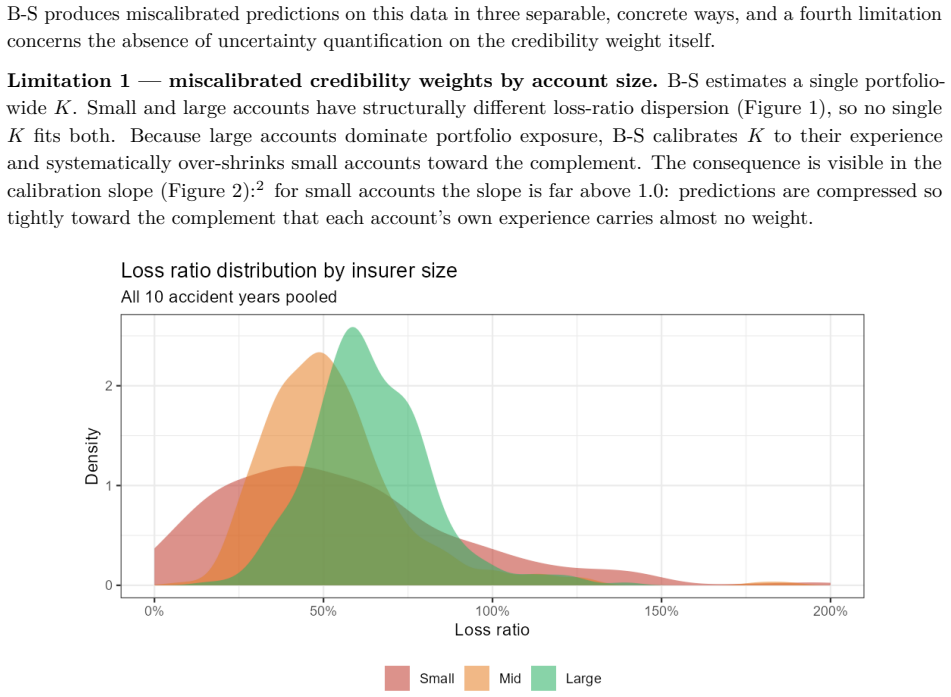
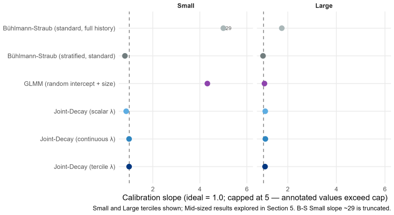
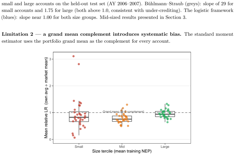
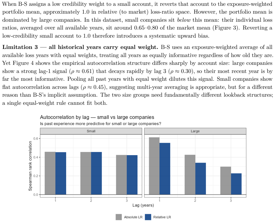
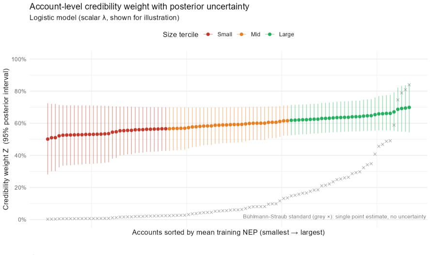
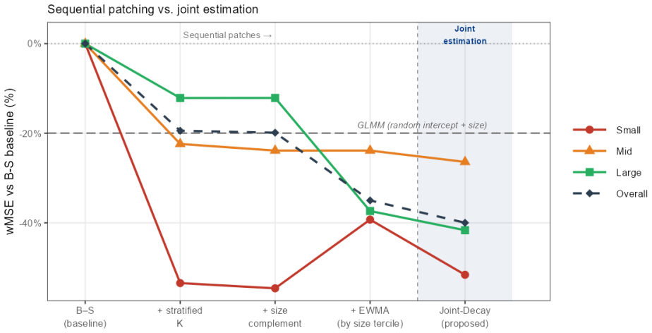
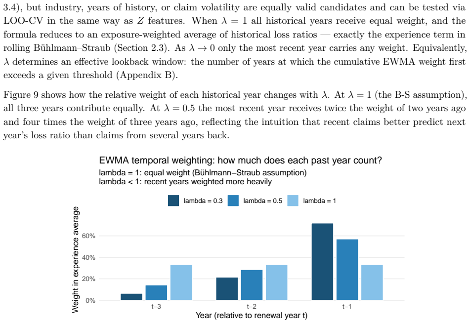
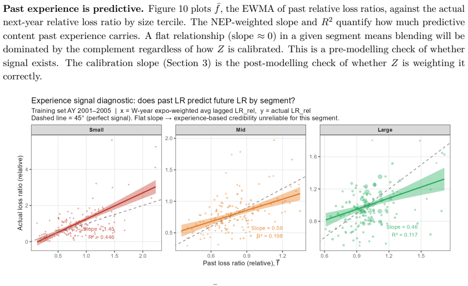
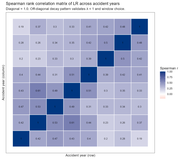
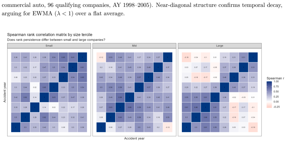
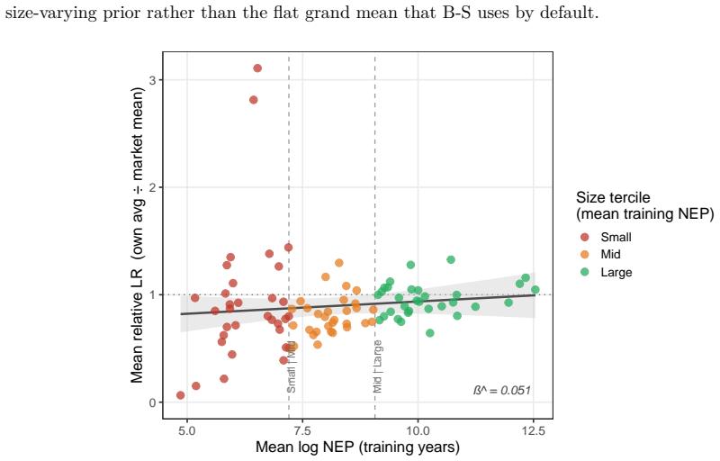
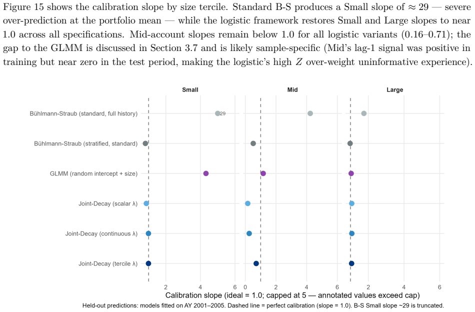
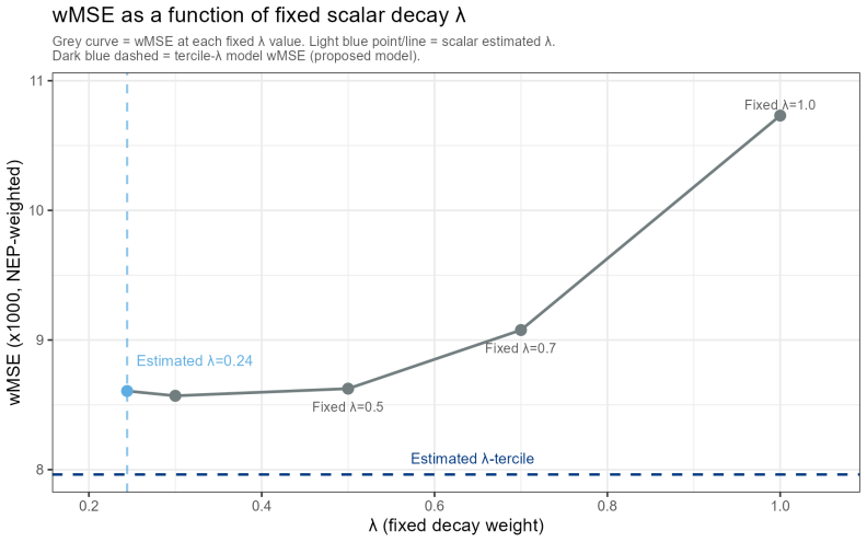
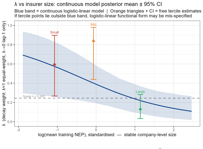
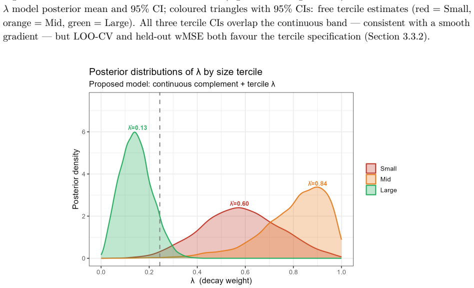
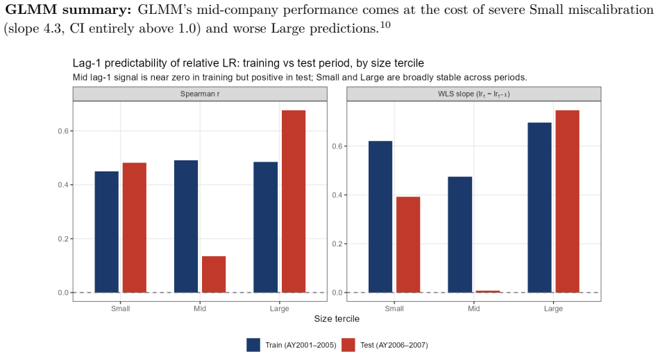
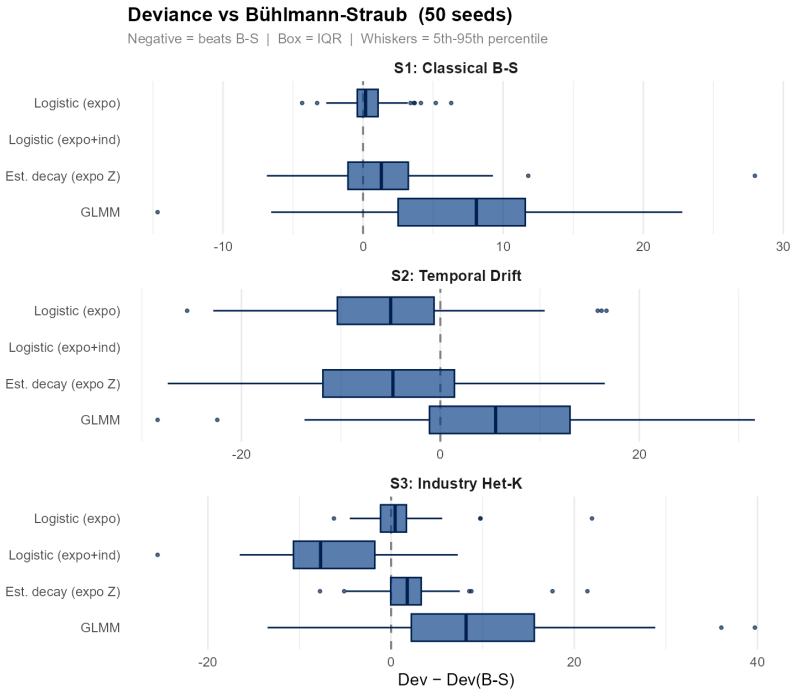
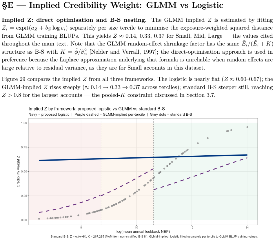
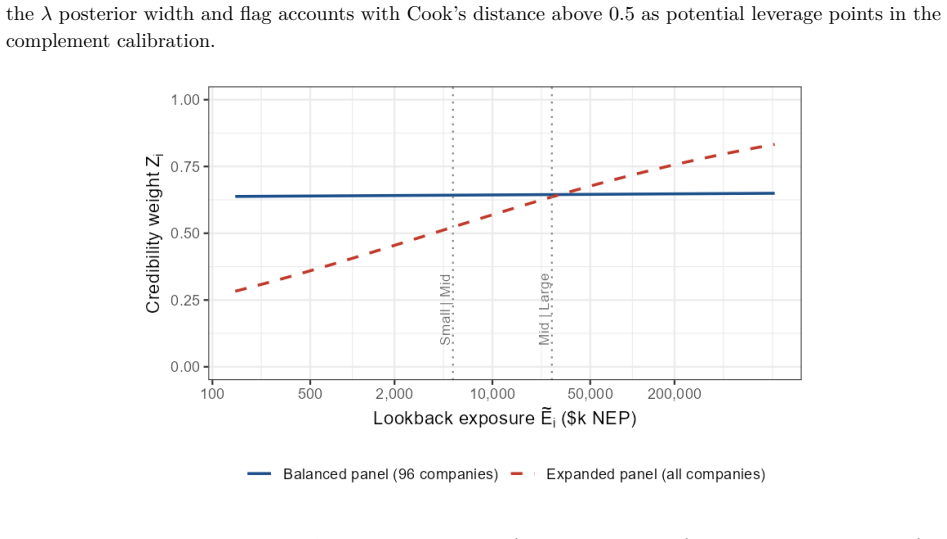
B\"uhlmann--Straub (B-S) credibility assigns each account a weight $Z_i = E_i/(E_i+K)$, where $K$ is a single portfolio-wide ratio. The formula assumes $K$ is the same for every account regardless of size, history length, or volatility, and that recent and older years carry equal weight. On a held-out US commercial auto dataset these assumptions fail: standard B-S applied to 96 companies produces a calibration slope of 29 for small accounts, a signature of severe under-crediting. We propose a joint framework that retains B-S interpretability while addressing these limitations. The credibility weight $Z_i$ is modelled as a logistic function of account characteristics; historical experience is discounted by an EWMA decay parameter $\lambda$ estimated from the data; and $Z$, $\lambda$, and the complement are optimised in a single likelihood pass. The framework formally nests B\"uhlmann--Straub as a special case, admitting a likelihood-ratio test for any proposed extension. On a two-year held-out test set the proposed model restores calibration (slope = 1.00) and reduces exposure-weighted prediction error by 38% (90% bootstrap interval: 26%--50%). A size gradient in the decay rate emerges ($\hat\lambda \approx 0.6$, $0.84$, $0.13$ for Small, Mid, Large) and replicates qualitatively on Other Liability. A simulation study confirms the mechanisms. The model requires only account-year summaries and delivers three transparent outputs: credibility weight, complement, and recommended renewal rate.
Editorial analysis
A structured set of objections, weighed in public.
Referee Report
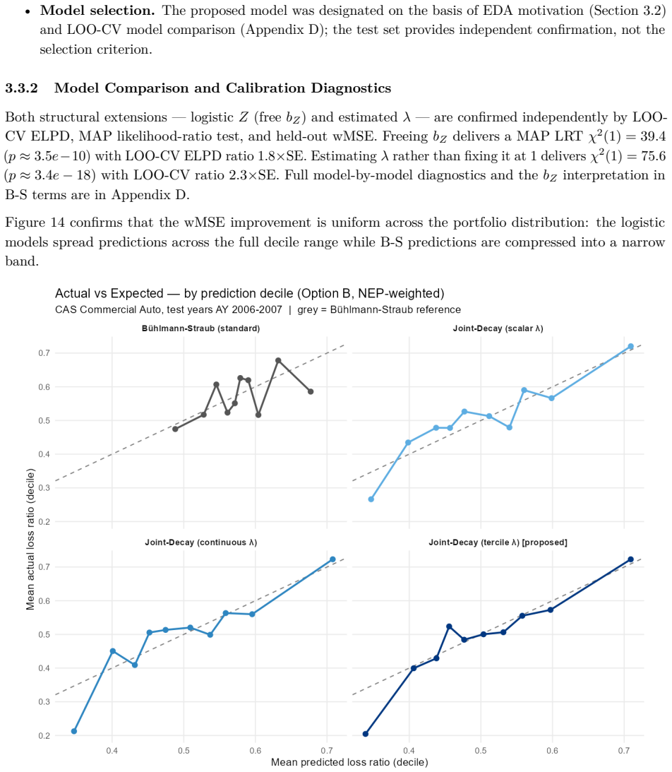
Summary. The paper extends Bühlmann-Straub credibility by replacing the fixed portfolio-wide K with a logistic function of account characteristics for the credibility weight Z_i, adding size-specific EWMA temporal decay rates λ estimated from data, and optimizing Z, λ, and the complement jointly via a single likelihood. The model nests standard B-S as a special case (admitting a likelihood-ratio test) and is evaluated on a two-year held-out US commercial auto dataset, where it reports restored calibration (slope = 1.00) and a 38% reduction in exposure-weighted prediction error (90% bootstrap interval 26%–50%), together with a size gradient in the estimated decay rates.
Significance. If the held-out results hold, the work supplies a practical, interpretable refinement of credibility theory for commercial lines that directly addresses the documented failures of constant-K and equal-history weighting. Credit is due for the explicit nesting of B-S, the use of a disjoint held-out test set with bootstrap intervals on both calibration slope and error reduction, the simulation study confirming mechanisms, and the requirement of only account-year summaries while producing transparent outputs (credibility weight, complement, renewal rate).
major comments (2)
- [Abstract] Abstract: the joint single-pass MLE of logistic coefficients together with three size-specific λ values (Small/Mid/Large) is presented without regularization, effective degrees of freedom, or the number of account characteristics; this makes the headline held-out claims (slope = 1.00 and 38% error reduction) vulnerable to optimistic bias from finite-sample noise in the training accounts.
- [Abstract] Abstract: the exact likelihood formulation, data exclusion rules, and definition of the size bands are not supplied, so the reported calibration and error metrics on the held-out set cannot be fully reconstructed or stress-tested for misspecification.
minor comments (1)
- The reported point estimates λ̂ ≈ 0.6, 0.84, 0.13 lack standard errors or intervals, which would strengthen the claim of a replicable size gradient.
Simulated Author's Rebuttal
We thank the referee for the constructive comments. Both major comments correctly identify information that is absent from the abstract. We will revise the abstract (and ensure the main text is explicit) to supply the missing details. Point-by-point responses follow.
read point-by-point responses
-
Referee: [Abstract] Abstract: the joint single-pass MLE of logistic coefficients together with three size-specific λ values (Small/Mid/Large) is presented without regularization, effective degrees of freedom, or the number of account characteristics; this makes the headline held-out claims (slope = 1.00 and 38% error reduction) vulnerable to optimistic bias from finite-sample noise in the training accounts.
Authors: We agree the abstract should state the number of account characteristics entering the logistic model. The manuscript uses unregularized maximum likelihood; the explicit nesting inside Bühlmann–Straub permits a likelihood-ratio test that guards against gratuitous complexity. The primary safeguard against optimistic bias is the disjoint two-year held-out test set together with bootstrap intervals on both calibration slope and error reduction. We will add the number of characteristics and a brief note on the absence of regularization to the revised abstract. revision: yes
-
Referee: [Abstract] Abstract: the exact likelihood formulation, data exclusion rules, and definition of the size bands are not supplied, so the reported calibration and error metrics on the held-out set cannot be fully reconstructed or stress-tested for misspecification.
Authors: The referee is correct that these elements are not stated in the abstract. The full manuscript defines the likelihood (the standard Bühlmann–Straub form with logistic Z and EWMA decay), the account-year data filters, and the exposure-based size bands (Small/Mid/Large). We will insert concise references to these definitions in the revised abstract so that the held-out metrics can be reconstructed from the text alone. revision: yes
Circularity Check
No significant circularity; held-out metrics independent of fitting equations
full rationale
The paper defines Z_i as logistic(account characteristics) and introduces size-specific EWMA decay rates λ estimated jointly with the logistic coefficients and complement via single likelihood on training accounts. The headline results (slope = 1.00, 38% error reduction) are reported on a disjoint two-year held-out test set whose observations do not enter the likelihood equations. The nesting of B-S as a special case is a formal restriction (λ = 0 or equivalent) that permits a likelihood-ratio test but does not make the test-set metrics tautological. No self-citation chain, uniqueness theorem, or ansatz imported from prior work is invoked to justify the central performance claims. The derivation therefore remains self-contained against external benchmarks.
Axiom & Free-Parameter Ledger
free parameters (2)
- logistic coefficients for Z
- EWMA decay rates lambda
axioms (2)
- domain assumption Bühlmann-Straub is recovered exactly when the logistic is constant and lambda equals 1
- domain assumption Account-year summaries contain sufficient information for stable likelihood estimation
Reference graph
Works this paper leans on
-
[1]
Catalina Bolançé, Montserrat Guillén, and Jean Pinquet
doi: 10.1016/j.insmatheco.2006.02.013. Catalina Bolançé, Montserrat Guillén, and Jean Pinquet. Time-varying credibility for frequency risk models: estimation and tests for autoregressive specifications on the random effects.Insurance: Mathematics and Economics, 33(2):273–282,
-
[2]
doi: 10.1016/S0167-6687(03)00139-2. R. L. Bornhuetter and R. E. Ferguson. The actuary and IBNR.Proceedings of the Casualty Actuarial Society, 59:181–195,
-
[3]
Hans Bühlmann and Erwin Straub
doi: 10.1007/3-540-29273-X. Hans Bühlmann and Erwin Straub. Glaubwürdigkeit für schadensätze.Mitteilungen der Vereinigung Schweizerischer Versicherungsmathematiker, 70:111–133,
-
[4]
Multilevel calibration weighting for survey data
doi: 10.18637/jss.v080.i01. Edward W. Frees, Virginia R. Young, and Yu Luo. A longitudinal data analysis interpretation of credibility models.Insurance: Mathematics and Economics, 24(3):229–247,
-
[5]
Strictly Proper Scoring Rules, Prediction, and Estimation , volume =
doi: 10.1198/016214506000001437. Charles A. Hachemeister. Credibility for regression models with application to trend. pages 129–163,
-
[6]
R Core Team.R: A Language and Environment for Statistical Computing
doi: 10.2143/AST.27.1.542963. R Core Team.R: A Language and Environment for Statistical Computing. R Foundation for Statistical Computing, Vienna, Austria,
-
[7]
Bjørn Sundt
URL https://mc-stan.org. Bjørn Sundt. A multi-level hierarchical credibility regression model.Scandinavian Actuarial Journal, 1980(1): 25–32,
1980
-
[8]
doi: 10.1080/03461238.1980.10408635. Bjørn Sundt. Credibility estimators with geometric weights.Insurance: Mathematics and Economics, 7(2): 113–122,
-
[9]
doi: 10.1016/0167-6687(88)90104-7. Aad W. van der Vaart.Asymptotic Statistics. Cambridge Series in Statistical and Probabilistic Mathematics. Cambridge University Press, Cambridge,
-
[10]
doi: 10.1007/s11222-016-9696-4. 50 §A — Nesting Proof and Rolling Bühlmann–Straub Exposition MLE Consistency Under the B-S Data-Generating Process Proposition (MLE recovery under a B-S data-generating process).Suppose the data are generated by the B-S mechanism with true structural parameterK0: that is, the true credibility weight isZi =wi/(wi+K0), the co...
-
[11]
5.7] under mild regularity conditions (compact parameter space, uniform law of large numbers)
Consistency of the sample estimator then follows from standard M-estimation results [van der Vaart, 2000, Thm. 5.7] under mild regularity conditions (compact parameter space, uniform law of large numbers). The compact parameter space condition is satisfied in any finite portfolio: log-exposurelog ˜Ei is bounded above by the largest account and below by th...
2000
-
[12]
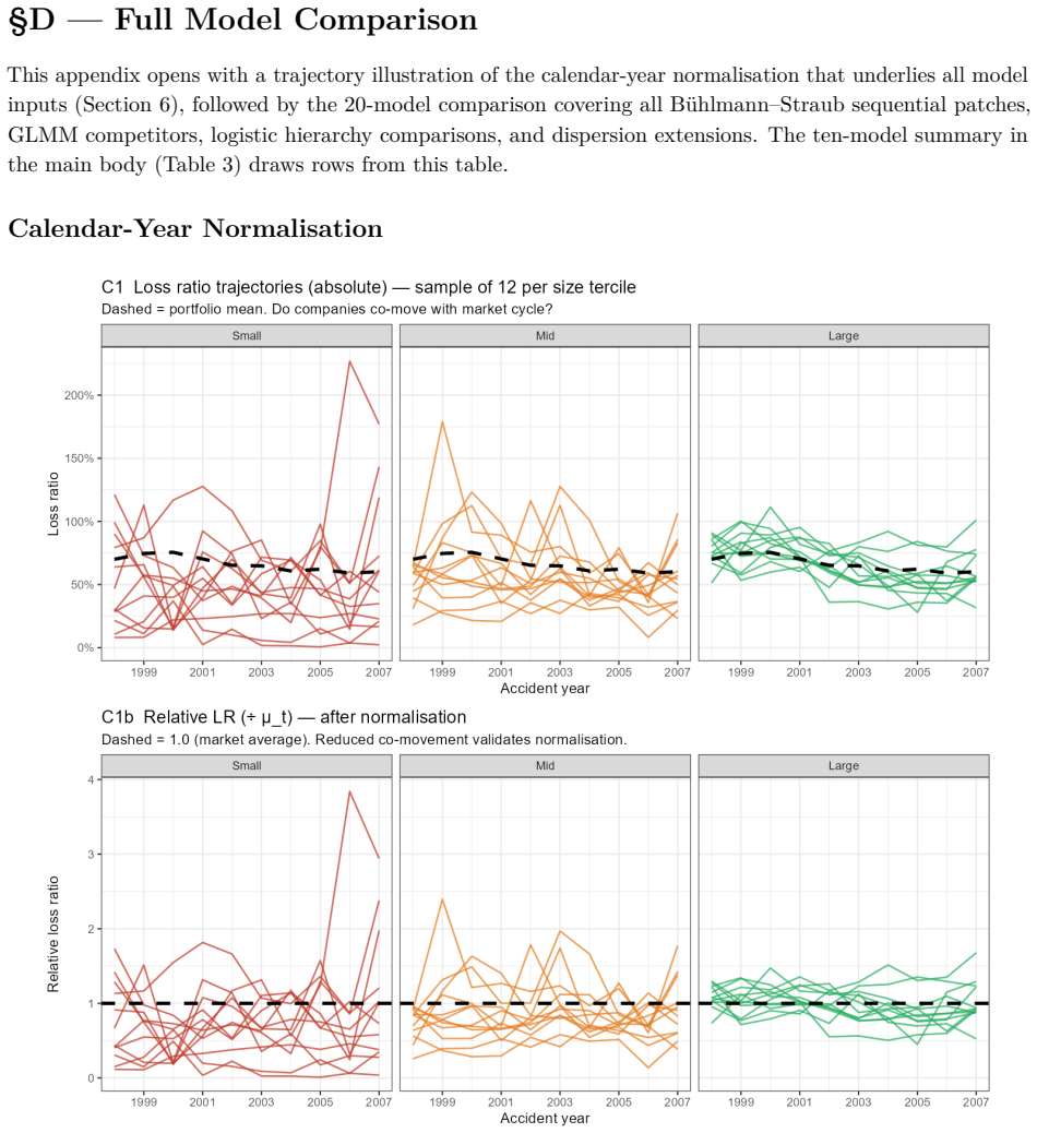
draws rows from this table. Calendar-Year Normalisation Figure 27: Loss ratio trajectories for a random sample of 12 companies per size tercile (same seed), before (upper panels) and after (lower panels) calendar-year normalisation. Dashed line = portfolio mean (upper) or 1.0 (lower). The elevated loss-ratio period (AY 2001–2002) is visible in all absolut...
2001
-
[13]
Small") df_train$is_md <-as.numeric(df_train$tercile==
fit_mle <-nlminb(init, nll, df = df_train, control =list(iter.max = 500, rel.tol = 1e-9)) par_hat <-setNames(fit_mle$par,names(init)) Listing 2: Bayesian Fit (brms) The brmsformula implements the recommended Joint-Decay tercile-λspecification (Equations 4–5), estimating one freeλper size tercile. Input data should contain one row per account-year with col...
2000
discussion (0)
Sign in with ORCID, Apple, or X to comment. Anyone can read and Pith papers without signing in.