REVIEW 3 major objections 4 minor 160 references
A modified transformer-based diffusion model can both fill in and forecast hydrological time series, with weather covariates sharpening event-driven predictions.
Reviewed by Pith at T0; open to challenge. T0 means a machine referee read the full paper against a public rubric. the ladder, T0–T4 →
T0 review · deepseek-v4-flash
2026-08-01 08:08 UTC pith:ZKRHM7KG
load-bearing objection A genuinely useful engineering adaptation of CSDI to hydrology, with a solid ablation study and honest limitations — but the headline claim of consistent superiority is contradicted by its own Table 16a, and the forecasting evaluation leaks future information via reanalysis covariates. the 3 major comments →
Transformer-based Diffusion models for Hydrological Time Series Probabilistic Imputation and Forecasting
The pith
A machine-rendered reading of the paper's core claim, the machinery that carries it, and where it could break.
Core claim
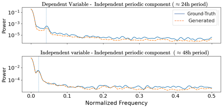
The central claim is that the proposed custom CSDI model — a transformer-based denoising diffusion network with added multi-scale convolutions, multiplicative-and-additive conditioning, root-mean-square normalization, and explicit Fourier encoding of day, week, and season cycles — outperforms all tested baselines on imputation and forecasting for the OPE dataset and almost all baselines on the synthetic dataset. The authors demonstrate that the model reproduces the target periodicities in simulations, reconstructs the inter-station correlation structure better than the original CSDI (though with weaker negative correlations), and, when augmented with weather covariates, successfully reproduc
What carries the argument
The central object is CSDI (Conditional Score-based Diffusion), a denoising diffusion model whose transformer backbone is trained to predict the noise added to missing time-series values while conditioning on observed values. The custom version adds: residual U-blocks with multi-scale convolutions to capture local and global temporal patterns; a conditioning mechanism with multiplicative scaling and additive offset; root-mean-square normalization for training stability; explicit Fourier encoding of periodicities (1 day, 7 days, 30 days, 90 days, 365 days); and an optional secondary input channel carrying meteorological covariates. During training, random masking simulates missingness, and th
Load-bearing premise
The headline forecasting results for the covariate-augmented model assume the model sees perfect future weather (reanalysis data) during evaluation; with real uncertain weather forecasts, the reported advantage over the no-covariate model could shrink or disappear.
What would settle it
Run the covariate-augmented model with operational numerical weather forecasts over the same forecast horizons instead of reanalysis weather; if the RMSE and CRPS advantage over the no-covariate model disappears, the forecasting benefit rests on perfect knowledge of future weather. A second check: evaluate the model on sequences longer than 15 days to see whether its periodic and low-frequency reproduction holds outside the short windows tested.
If this is right
- A single diffusion model can serve both data imputation and probabilistic forecasting, removing the need for task-specific models at a monitoring network.
- Weather covariates as conditioning can substantially improve forecasting of event-driven shifts such as rain-driven stream peaks, pointing toward a data-driven alternative to purely autoregressive hydrological models.
- The model is well suited to imputing gaps of moderate size (around 100 synthetic timesteps) and short-term forecasting, but its advantage over classical Gaussian-process methods shrinks for longer gaps.
- The reproduced between-station correlation structure supports multisite simulation, though negative cross-variable correlations remain underestimated, limiting some joint water-quality predictions.
Where Pith is reading between the lines
- The forecasting gains of the covariate-augmented model were measured with reanalysis weather over the forecast horizon, so they are likely an upper bound: feeding the model real numerical weather forecasts, or ensembles of them, would show how much of the advantage survives operational uncertainty.
- The acknowledged weakness with negative correlations suggests a direct architectural test: replacing the softmax attention with a kernel that permits negative weights, such as cosFormer, could improve joint water-quality modeling without retraining the whole pipeline.
- A hybrid deployment that delegates long gaps to a statistical baseline could leverage the diffusion model's short-gap accuracy while compensating for its long-gap degradation.
- Because training data were corrected for sensor drift, real-time deployment on raw uncorrected sensor inputs is expected to degrade simulation quality; quantifying that degradation with a raw-data test would clarify operational limits.
Editorial analysis
A structured set of objections, weighed in public.
Referee Report
Summary. This paper proposes a modified Conditional Score-based Diffusion Model (CSDI) for probabilistic imputation and forecasting of multivariate hydrological time series. The modifications — residual U-blocks, convolutional layers, StyleGAN-style conditioning with RMSNorm, and Fourier periodic encodings — are motivated by observed failures of vanilla CSDI on the OPE dataset, and a covariate-augmented version adds meteorological covariates. The model is evaluated on a synthetic hydrology-like dataset and on a real 6-station, 13-variable water-quality/quantity dataset, against GP, original CSDI, U-Net, TSMixer, and NHits baselines, using RMSE, MAE, SMAPE, and CRPS, plus PSD and correlation-matrix diagnostics. The authors claim consistent superiority of the custom CSDI architecture, with covariate augmentation helping forecasting.
Significance. If the claims hold, this is a useful applied contribution: a single probabilistic model for both imputation and forecasting of multivariate, missing-data-heavy hydrological time series, with credible uncertainty bands and code availability. The step-by-step ablations (Appendix D) and the explicit synthetic generator (Appendix E) are valuable for reproducibility. The methodological novelty is incremental — the architecture is a composition of published components — and the real-data evaluation is limited; furthermore, the headline 'consistently outperforms all baselines' claim is internally contradicted by Table 16a. The contribution remains publishable after the claims are made metric-specific and the oracle-covariate issue is clearly labeled.
major comments (3)
- [§4.3, Table 16a] The claim 'across all metrics, the custom CSDI architecture (with and without covariates) consistently outperforms all baselines' is contradicted by Table 16a. At 25% missing values, the non-covariate Custom model has RMSE 0.1676±0.0049, while GP has 0.1609±0.0008; the custom model is therefore not strictly better than all baselines on this metric. Since the claim appears in Section 4.3 and is echoed elsewhere, it must be revised to a metric-specific or majority-of-metrics formulation, or the table corrected.
- [§3.1, §4.1, §5] The covariate-augmented model is trained and evaluated with SAFRAN reanalysis covariates over the full forecast horizon. Reanalysis is a posterior product, not an available forecast, so the forecasting comparison gives the augmented model perfect future information that covariate-free baselines do not receive. The Discussion acknowledges this ('does not fully correspond to an operational forecasting setting'), but the headline forecasting advantage in Figures 8-9 remains operational unfalsified. Please relabel these results as an oracle/perfect-information upper bound, or add an experiment with lagged or forecast-error-perturbed covariates.
- [§4.1, §4.3] The real-data evaluation uses a test partition of only 28 elementary windows (and 20 validation windows), each 24 timesteps long. This is small for claiming 'consistently outperforms' across all metrics and horizons. Report per-window variability, confidence intervals, or a bootstrap over windows, and ensure the claim is not stronger than the effective sample size supports.
minor comments (4)
- [§4.1] The text says 'See Appendix 4 for an overview of the evaluation framework' but the detailed metrics are in Appendix F; the cross-reference should be corrected.
- [§2.2, Eq. (8)] Equation (8) has garbled formatting: the weighting term and the norm symbols are unclear. Please re-typeset and verify the expression.
- [§4.3, Figure 11] The Figure 11 caption says 'simulating 15 days given 16 days', whereas the evaluation setting in §4.1 describes 24-timestep windows and horizons of 6-12 timesteps at 4-hour resolution. Clarify whether Figure 11 uses a different experiment; otherwise this is an inconsistency.
- [Throughout] The name 'U-NET' is used inconsistently (U-Net, U-NET). Also 'Guigues et al., ress' in the references should be 'in press'.
Circularity Check
No significant circularity: the paper is an empirical ML evaluation with a standard diffusion objective; fixed Fourier features and non-load-bearing self-citation do not create a circular derivation.
full rationale
This is an empirical machine-learning benchmark, not a derivation chain, so the main circularity-by-construction failure mode does not arise. The diffusion training objective (Eq. 9) and the CSDI conditional loss (Eq. 12) are standard score-matching losses; the reported imputation and forecasting numbers are obtained by training on training data and evaluating on masked held-out test windows, so no reported metric is defined in terms of the fitted parameters. The Fourier timestep encoding in Section 3.1 is explicitly a fixed, hand-selected input representation: 'we use cycles of 1 day, 7 days, 30 days, 90 days and 365 days', described as 'predefined cycle lengths'; it is not fitted to the test labels, and the synthetic-data evaluation also reproduces a 48h period that is not among the injected Fourier cycles. The only self-citation, Bhavsar et al. (2024), is used to support the generic statement that GAN training 'often suffers from stability issues'; it is not load-bearing for any central claim. The covariate-augmented forecasting setup uses SAFRAN reanalysis over the forecast horizon, and the Discussion explicitly admits that this 'does not fully correspond to an operational forecasting setting'; that is an evaluation-validity limitation, not a circular step. Similarly, Table 16a at 25% missing values reports Custom RMSE 0.1676±0.0049 versus GP RMSE 0.1609±0.0008, which contradicts the text's claim that the custom architecture 'consistently outperforms all baselines'; this is an internal inconsistency or correctness issue, not a circular argument. No prediction in the paper reduces by construction to its input, so the circularity score is 0.
Axiom & Free-Parameter Ledger
free parameters (1)
- Fourier cycle lengths =
[1, 7, 30, 90, 365] days
axioms (4)
- standard math Diffusion reverse process can be approximated by a noise-prediction network (Ho et al. 2020)
- domain assumption OPEs data quality corrections (LNE/Andra) make the corrected measurements a reliable ground truth
- domain assumption SAFRAN reanalysis is a valid proxy for meteorological forecasting covariates
- domain assumption The synthetic dataset mimics the relevant hydrological dynamics of the real system
read the original abstract
The modeling of hydrometeorological time series with limited observations is a key challenge in the monitoring of hydro-systems and water resources, as well as for flood or drought risk assessment. Due to the high variability of the underlying processes and the sparsity of available measurements, traditional statistical approaches often struggle to accurately represent their dynamics. In this context, recent advances in deep learning offer a promising direction for improving the representation and generation of complex temporal processes sampled at several observation sites. This study investigates the application of transformer-based diffusion models to the simulation and reconstruction of hydrological time series. The proposed framework is applied to the joint modeling of water quantity and quality at six sites spread across three adjacent headwater catchments located in North-East France on a limestone plateau covered by forests and field crops. The model is calibrated and validated using available observational data, which has been quality controlled and corrected for sensor drift and malfunction through collaborative efforts by LNE metrology expertise and Andra monthly quality control over more than 15 years. Its performance is compared with several established baseline approaches commonly used for time series modeling. Quantitative evaluation metrics are employed to assess the ability of the proposed method to reproduce key temporal characteristics of the observed signals in two settings: the imputation of incomplete time series and the forecasting of upcoming hydrological conditions. Results support the effectiveness of the transformer-based approach and highlight its capacity to capture and simulate the complex patterns present in hydrological data. In particular, the results indicate that diffusion models can efficiently sample realistic time series distributions under observation settings with variable missing data for both forecasting and imputation.
Figures




Reference graph
Works this paper leans on
-
[1]
Alcaraz, J. M. L. and N. Strodthoff (2023). Diffusion-based time series imputation and forecasting with structured state space models
2023
-
[2]
Allcroft, D. J. and C. A. Glasbey (2003, 09). A latent gaussian markov random-field model for spatiotemporal rainfall disaggregation. Journal of the Royal Statistical Society Series C: Applied Statistics\/ 52\/ (4), 487--498
2003
-
[3]
Alornyo, S. A., W. R. McGillis, and P. J. Culligan (2026). From sensors to simulations: How ai is transforming water monitoring, management, and policy. Water\/ 18\/ (14)
2026
-
[5]
Chintala, and L
Arjovsky, M., S. Chintala, and L. Bottou (2017). Wasserstein generative adversarial networks. In International conference on machine learning , pp.\ 214--223. PMLR
2017
-
[6]
Cho, and Y
Bahdanau, D., K. Cho, and Y. Bengio (2015). Neural machine translation by jointly learning to align and translate. In Proceedings of the 3rd International Conference on Learning Representations (ICLR 2015)
2015
-
[7]
Balaji, and Z
Bansal, A., K. Balaji, and Z. Lalani (2025). Temporal encoding strategies for energy time series prediction
2025
-
[8]
Janati, G
Bedin, L., Y. Janati, G. Victorino Cardoso, J. Duchateau, R. Dubois, and E. Moulines (2025, 06). Reconstructing ecg from indirect signals: a denoising diffusion approach. Philosophical Transactions of the Royal Society A: Mathematical, Physical and Engineering Sciences\/ 383\/ (2299), 20240330
2025
-
[9]
Desassis, F
Bhavsar, F., N. Desassis, F. Ors, and T. Romary (2024). A stable deep adversarial learning approach for geological facies generation. Computers & Geosciences\/ 190 , 105638
2024
-
[10]
Donahue, and K
Brock, A., J. Donahue, and K. Simonyan (2019). Large scale GAN training for high fidelity natural image synthesis
2019
-
[11]
Brunner, M. I., A. B\'ardossy, and R. Furrer (2019). Technical note: Stochastic simulation of streamflow time series using phase randomization. Hydrology and Earth System Sciences\/ 23\/ (8), 3175--3187
2019
-
[12]
C. M., N. and N. Thangarasu (2025, 11). Enhancing dam inflow forecasting using hybrid deep learning and diffusion models: a case study on the malampuzha dam. Water Practice and Technology\/ 20\/ (11), 2276--2293
2025
-
[13]
Challu, C., K. G. Olivares, B. N. Oreshkin, F. Garza, M. Mergenthaler-Canseco, and A. Dubrawski (2022). N-hits: Neural hierarchical interpolation for time series forecasting
2022
-
[14]
Chen, C., F. Wang, Z. Wang, D. Zhang, and L. Xiang (2025, June). A novel flood forecasting model based on TimeGAN for data-sparse basins. Stochastic Environmental Research and Risk Assessment\/ 39\/ (6), 2267--2280
2025
-
[15]
Chen, S.-A., C.-L. Li, N. Yoder, S. O. Arik, and T. Pfister (2023). Tsmixer: An all-mlp architecture for time series forecasting
2023
-
[16]
Cybenko, G. (1989). Approximation by superpositions of a sigmoidal function. Mathematics of control, signals and systems\/ 2\/ (4), 303--314
1989
-
[17]
Dhariwal, P. and A. Nichol (2021). Diffusion models beat gans on image synthesis. In M. Ranzato, A. Beygelzimer, Y. Dauphin, P. Liang, and J. W. Vaughan (Eds.), Advances in Neural Information Processing Systems , Volume 34, pp.\ 8780--8794. Curran Associates, Inc
2021
-
[18]
Dieleman, S., L. Sartran, A. Roshannai, N. Savinov, Y. Ganin, P. H. Richemond, A. Doucet, R. Strudel, C. Dyer, C. Durkan, C. Hawthorne, R. Leblond, W. Grathwohl, and J. Adler (2022). Continuous diffusion for categorical data. ArXiv\/ abs/2211.15089
Pith/arXiv arXiv 2022
-
[19]
Fang, and C
Feng, D., K. Fang, and C. Shen (2020, September). Enhancing streamflow forecast and extracting insights using long‐short term memory networks with data integration at continental scales. Water Resources Research\/ 56\/ (9)
2020
-
[20]
Pouget-Abadie, M
Goodfellow, I., J. Pouget-Abadie, M. Mirza, B. Xu, D. Warde-Farley, S. Ozair, A. Courville, and Y. Bengio (2014). Generative adversarial nets. In Advances in neural information processing systems , pp.\ 2672--2680
2014
-
[21]
Goodfellow, I. J., Y. Bengio, and A. Courville (2016). Deep Learning . Cambridge, MA, USA: MIT Press. http://www.deeplearningbook.org
2016
-
[22]
Gu, S., D. Chen, J. Bao, F. Wen, B. Zhang, D. Chen, L. Yuan, and B. Guo (2022, June). Vector quantized diffusion model for text-to-image synthesis. In Proceedings of the IEEE/CVF Conference on Computer Vision and Pattern Recognition (CVPR) , pp.\ 10696--10706
2022
-
[23]
Guardiano, F. and M. Srivastava (1993). Multivariate geostatistics: Beyond bivariate moments. In A. Soares (Ed.), Geostatistics Troia , pp.\ 133--144. Dordrecht: Kluwer Academic Publications
1993
-
[24]
Savatier, and B
Guigues, N., M. Savatier, and B. Lalère (in press). Quantifying measurement uncertainty in real time continuous water quality monitoring: methodological approaches and implications for data interpretation. Environmental Science: Processes & Impacts\/ . In press
-
[25]
Lintern, J
Guo, D., A. Lintern, J. A. Webb, D. Ryu, U. Bende-Michl, S. Liu, and A. W. Western (2020). A data-based predictive model for spatiotemporal variability in stream water quality. Hydrology and Earth System Sciences\/ 24\/ (2), 827--847
2020
-
[26]
He, J., Y.-J. Chen, A. Jafari, A. Idamekorala, and G. Fox (2025). Deep learning foundation and pattern models: Challenges in hydrological time series
2025
-
[27]
Zhang, S
He, K., X. Zhang, S. Ren, and J. Sun (2015). Deep residual learning for image recognition
2015
-
[28]
Lässig, S
Herzen, J., F. Lässig, S. G. Piazzetta, T. Neuer, L. Tafti, G. Raille, T. V. Pottelbergh, M. Pasieka, A. Skrodzki, N. Huguenin, M. Dumonal, J. Kościsz, D. Bader, F. Gusset, M. Benheddi, C. Williamson, M. Kosinski, M. Petrik, and G. Grosch (2022). Darts: User-friendly modern machine learning for time series. Journal of Machine Learning Research\/ 23\/ (124), 1--6
2022
-
[30]
Hochreiter, S. and J. Schmidhuber (1997, 12). Long short-term memory. Neural computation\/ 9 , 1735--80
1997
-
[31]
Hu, J., P. Wang, D. Li, and S. Liu (2024). A long-term multivariate time series prediction model for dissolved oxygen. Ecological Informatics\/ 82 , 102695
2024
-
[32]
Noutahi, J
Jones, C., E. Noutahi, J. Hartford, and C. Eastwood (2026). Elucidating the design space of flow matching for cellular microscopy
2026
-
[33]
Laine, and T
Karras, T., S. Laine, and T. Aila (2019). A style-based generator architecture for generative adversarial networks. In Proceedings of the IEEE/CVF conference on computer vision and pattern recognition , pp.\ 4401--4410
2019
-
[34]
Kawar, B., S. Zada, O. Lang, O. Tov, H. Chang, T. Dekel, I. Mosseri, and M. Irani (2023, June). Imagic: Text-based real image editing with diffusion models. In Proceedings of the IEEE/CVF Conference on Computer Vision and Pattern Recognition (CVPR) , pp.\ 6007--6017
2023
-
[35]
Kingma, D. P. and M. Welling (2014). Auto-encoding variational bayes
2014
-
[36]
Klotz, C
Kratzert, F., D. Klotz, C. Brenner, K. Schulz, and M. Herrnegger (2018). Rainfall--runoff modelling using long short-term memory (lstm) networks. Hydrology and Earth System Sciences\/ 22\/ (11), 6005--6022
2018
-
[37]
Li, C., X. Ling, Y. Xue, W. Luo, L. Zhu, F. Qin, Y. Zhou, and Y. Huang (2024). Precipitation nowcasting using diffusion transformer with causal attention. IEEE Transactions on Geoscience and Remote Sensing\/ 62 , 1--16
2024
-
[38]
Renard, and J
Mariethoz, G., P. Renard, and J. Straubhaar (2010). The direct sampling method to perform multiple-point geostatistical simulations. Water Resources Research\/ 46\/ (11)
2010
-
[40]
Royer, D
Moiroux-Arvis, L., L. Royer, D. Sarramia, G. De Sousa, A. Claude, D. Latour, E. Roussel, O. Voldoire, P. Chardon, R. Vanda \"e le, et al. (2023). Connecsens, a versatile iot platform for environment monitoring: Bring water to cloud. Sensors\/ 23\/ (6), 2896
2023
-
[42]
Benoit, and D
Obakrim, S., L. Benoit, and D. Allard (2025). A multivariate and space-time stochastic weather generator using a latent gaussian framework. Stochastic Environmental Research and Risk Assessment\/ 39\/ (9), 3677--3701
2025
-
[43]
Ou, Z., C. Nai, B. Pan, Y. Zheng, C. Shen, P. Jiang, X. Liu, Q. Tang, W. Li, and M. Pan (2025, July). Probabilistic diffusion models advance extreme flood forecasting. Geophysical Research Letters\/ 52\/ (15)
2025
-
[44]
Peebles, W. and S. Xie (2023). Scalable diffusion models with transformers
2023
-
[45]
Zhang, C
Qin, X., Z. Zhang, C. Huang, M. Dehghan, O. R. Zaiane, and M. Jagersand (2020). U2-net: Going deeper with nested u-structure for salient object detection. Pattern recognition\/ 106 , 107404
2020
-
[46]
Qin, Z., W. Sun, H. Deng, D. Li, Y. Wei, B. Lv, J. Yan, L. Kong, and Y. Zhong (2022). cosformer: Rethinking softmax in attention
2022
-
[47]
Le Moigne, Y
Quintana-Segui, P., P. Le Moigne, Y. Durand, E. Martin, F. Habets, M. Baillon, C. Canellas, L. Franchisteguy, and S. Morel (2008). Analysis of near-surface atmospheric variables: V alidation of the SAFRAN analysis over F rance. Journal of Applied Meteorology and Climatology\/ 47\/ (1), 92--107
2008
-
[48]
Saeed, M
Rashid, M., A. Saeed, M. Khalid, A. Murtaza, and M. Waqar Saleem (2026). The transformative role of artificial intelligence in water resources engineering: A comprehensive review. Environmental Modelling & Software\/ 197 , 106857
2026
-
[49]
Rattanatheerawon, W. and R. Fooprateepsiri (2025). Diffusion-driven time-series forecasting to support sustainable river ecosystems and sdg-aligned water-resource governance in thailand. Sustainability\/ 17\/ (22)
2025
-
[50]
Cromwell, B
Ren, H., E. Cromwell, B. Kravitz, and X. Chen (2022). Technical note: Using long short-term memory models to fill data gaps in hydrological monitoring networks. Hydrology and Earth System Sciences\/ 26\/ (7), 1727--1743
2022
-
[51]
Fischer, and T
Ronneberger, O., P. Fischer, and T. Brox (2015). U-net: Convolutional networks for biomedical image segmentation. In Medical Image Computing and Computer-Assisted Intervention--MICCAI 2015: 18th International Conference, Munich, Germany, October 5-9, 2015, Proceedings, Part III 18 , pp.\ 234--241. Springer
2015
-
[52]
Ruiz, N., Y. Li, V. Jampani, Y. Pritch, M. Rubinstein, and K. Aberman (2023, June). Dreambooth: Fine tuning text-to-image diffusion models for subject-driven generation. In Proceedings of the IEEE/CVF Conference on Computer Vision and Pattern Recognition (CVPR) , pp.\ 22500--22510
2023
-
[53]
Saharia, C., W. Chan, H. Chang, C. Lee, J. Ho, T. Salimans, D. Fleet, and M. Norouzi (2022a). Palette: Image-to-image diffusion models. In ACM SIGGRAPH 2022 Conference Proceedings , SIGGRAPH '22, New York, NY, USA. Association for Computing Machinery
2022
-
[54]
Saharia, C., W. Chan, H. Chang, C. A. Lee, J. Ho, T. Salimans, D. J. Fleet, and M. Norouzi (2022b). Palette: Image-to-image diffusion models
-
[55]
Shevnina, E. and A. Silaev (2019). The probabilistic hydrological marcs ^HYDRO (the markov chain system) model: its structure and core version 0.2. Geoscientific Model Development\/ 12\/ (7), 2767--2780
2019
-
[56]
Sohl-Dickstein, J., E. A. Weiss, N. Maheswaranathan, and S. Ganguli (2015). Deep unsupervised learning using nonequilibrium thermodynamics
2015
-
[57]
Strebelle, S. and A. G. Journel (2000). Sequential Simulation Drawing Structures from Training Images . Dissertation
2000
-
[58]
Tashiro, Y., J. Song, Y. Song, and S. Ermon (2021). Csdi: Conditional score-based diffusion models for probabilistic time series imputation. In M. Ranzato, A. Beygelzimer, Y. Dauphin, P. Liang, and J. W. Vaughan (Eds.), Advances in Neural Information Processing Systems , Volume 34, pp.\ 24804--24816. Curran Associates, Inc
2021
-
[59]
van Wijk , W
Teurlincx, S., D. van Wijk , W. M. Mooij, J. J. Kuiper, I. Huttunen, R. J. Brederveld, M. Chang, J. H. Janse, B. Woodward, F. Hu, and A. B. Janssen (2019). A perspective on water quality in connected systems: modelling feedback between upstream and downstream transport and local ecological processes. Current Opinion in Environmental Sustainability\/ 40 , ...
2019
-
[60]
(2016, 03)
Tunnicliffe Wilson, G. (2016, 03). Time series analysis: Forecasting and control,5th edition, by george e. p. box, gwilym m. jenkins, gregory c. reinsel and greta m. ljung, 2015. published by john wiley and sons inc., hoboken, new jersey, pp. 712. isbn: 978-1-118-67502-1. Journal of Time Series Analysis\/ 37 , n/a--n/a
2016
-
[61]
Shazeer, N
Vaswani, A., N. Shazeer, N. Parmar, J. Uszkoreit, L. Jones, A. N. Gomez, L. Kaiser, and I. Polosukhin (2023). Attention is all you need
2023
-
[62]
Studer, and J
von Freyberg, J., B. Studer, and J. W. Kirchner (2017). A lab in the field: high-frequency analysis of water quality and stable isotopes in stream water and precipitation. Hydrology and Earth System Sciences\/ 21\/ (3), 1721--1739
2017
-
[63]
Zhang, S
Wang, Q., J. Zhang, S. Song, and Z. Zhang (2014). Attentional neural network: Feature selection using cognitive feedback. In Advances in Neural Information Processing Systems (NIPS 2014)
2014
-
[64]
Zhang, P
Wang, X., H. Zhang, P. Wang, Y. Zhang, B. Wang, Z. Zhou, and Y. Wang (2023). An observed value consistent diffusion model for imputing missing values in multivariate time series. In Proceedings of the 29th ACM SIGKDD Conference on Knowledge Discovery and Data Mining , KDD '23, New York, NY, USA, pp.\ 2409–2418. Association for Computing Machinery
2023
-
[65]
Kojima (2022)
Weilisi and T. Kojima (2022). Investigation of hyperparameter setting of a long short-term memory model applied for imputation of missing discharge data of the daihachiga river. Water\/ 14\/ (2)
2022
-
[66]
Wang, and X
Yang, C., T. Wang, and X. Yan (2023). Ddmt: Denoising diffusion mask transformer models for multivariate time series anomaly detection
2023
-
[67]
Yang, D., J. Yu, H. Wang, W. Wang, C. Weng, Y. Zou, and D. Yu (2023). Diffsound: Discrete diffusion model for text-to-sound generation. IEEE/ACM Transactions on Audio, Speech, and Language Processing\/ 31 , 1720--1733
2023
-
[68]
Yuan, X. and Y. Qiao (2024). Diffusion-ts: Interpretable diffusion for general time series generation
2024
-
[69]
Zhang, B. and R. Sennrich (2019). Root mean square layer normalization . Red Hook, NY, USA: Curran Associates Inc
2019
-
[70]
Zhang, H., J. Zhou, Y. Lu, M. Guo, P. Wang, L. Shen, and Q. Qu (2024). The emergence of reproducibility and generalizability in diffusion models
2024
-
[71]
Rao, and M
Zhang, L., A. Rao, and M. Agrawala (2023, October). Adding conditional control to text-to-image diffusion models. In Proceedings of the IEEE/CVF International Conference on Computer Vision (ICCV) , pp.\ 3836--3847
2023
-
[72]
Zhu, J.-Y., T. Park, P. Isola, and A. A. Efros (2020). Unpaired image-to-image translation using cycle-consistent adversarial networks
2020
-
[73]
Generative Adversarial Networks , volume =
Goodfellow, Ian and Pouget-Abadie, Jean and Mirza, Mehdi and Xu, Bing and Warde-Farley, David and Ozair, Sherjil and Courville, Aaron and Bengio, Yoshua , year =. Generative Adversarial Networks , volume =. Advances in Neural Information Processing Systems , doi =
-
[74]
Denoising Diffusion Probabilistic Models , url =
Ho, Jonathan and Jain, Ajay and Abbeel, Pieter , booktitle =. Denoising Diffusion Probabilistic Models , url =
-
[75]
Diffusion Models Beat GANs on Image Synthesis , url =
Dhariwal, Prafulla and Nichol, Alexander , booktitle =. Diffusion Models Beat GANs on Image Synthesis , url =
-
[76]
Time Series Analysis: Forecasting and Control,5th Edition, by George E
Tunnicliffe Wilson, Granville , year =. Time Series Analysis: Forecasting and Control,5th Edition, by George E. P. Box, Gwilym M. Jenkins, Gregory C. Reinsel and Greta M. Ljung, 2015. Published by John Wiley and Sons Inc., Hoboken, New Jersey, pp. 712. ISBN: 978-1-118-67502-1 , volume =. Journal of Time Series Analysis , doi =
2015
-
[77]
Can a Training Image Be a Substitute for a Random Field Model? , volume =
Emery, Xavier and Lantuéjoul, Christian , year =. Can a Training Image Be a Substitute for a Random Field Model? , volume =. Mathematical Geosciences , doi =
-
[78]
Alessandro Comunian and Sanjeev K. Jha and Beatrice M. S. Giambastiani and Gregoire Mariethoz and Bryce F. J. Kelly , title =. Mathematical Geosciences , year =. doi:10.1007/s11004-013-9505-y , url =
-
[79]
and Srivastava, M
Guardiano, F. and Srivastava, M. , title =. Geostatistics Troia , editor =. 1993 , publisher =
1993
-
[80]
, title =
Strebelle, Sebastien and Journel, Andree G. , title =. 2000 , type =
2000
-
[81]
Matheron, Georges and Pawlowsky-Glahn, Vera and Serra, Jean , isbn =. 1Introduction. Matheron's Theory of Regionalised Variables. 2019 , month =. doi:10.1093/oso/9780198835660.003.0001 , url =
arXiv 2019
-
[82]
J. P. Chil\`es and P. Delfiner. Geostatistics, M odeling S patial U ncertainty
-
[83]
M. Armstrong , title =. Journal of the International Association for Mathematical Geology , year =. doi:10.1007/BF01036241 , url =
-
[84]
arXiv preprint arXiv:1701.04862 , year=
Towards principled methods for training generative adversarial networks , author=. arXiv preprint arXiv:1701.04862 , year=
discussion (0)
Sign in with ORCID, Apple, or X to comment. Anyone can read and Pith papers without signing in.