pith. sign in

arxiv: 2212.08989 · v3 · pith:CAVQMFLSnew · submitted 2022-12-18 · 💻 cs.LG

Deep learning applied to computational mechanics: A comprehensive review, state of the art, and the classics

Pith reviewed 2026-05-24 10:19 UTC · model grok-4.3

classification 💻 cs.LG
keywords deep learningcomputational mechanicsphysics-informed neural networkshybrid methodsLSTMfinite element methodmodel order reductionconstitutive modeling
0
0 comments X

The pith

Deep learning methods, both hybrid and pure, are reviewed for use in solid and fluid mechanics simulations.

A machine-rendered reading of the paper's core claim, the machinery that carries it, and where it could break.

The paper establishes a detailed survey of how artificial neural networks and deep learning are applied to computational mechanics problems involving solids, fluids, and finite-element technology. It distinguishes hybrid approaches that combine traditional PDE discretizations with machine learning from pure machine learning methods such as physics-informed neural networks. The review builds DL concepts from the basics for readers already familiar with mechanics, while also covering LSTM architectures, attention mechanisms, optimizers, and kernel methods like Gaussian processes. A sympathetic reader would care because the survey aims to bring newcomers quickly to the research frontier and to correct misconceptions found even in well-known references on the history and limits of AI. The positioning and control of a large-deformable beam serves as a concrete example throughout.

Core claim

The paper claims that recent deep learning developments relevant to computational mechanics can be organized into hybrid methods, which use LSTM networks to model nonlinear constitutive relations or reduce model order and convolutional networks to accelerate traditional integrators, and pure ML methods represented by physics-informed neural networks that may incorporate attention to handle discontinuous solutions; it further reviews LSTM and attention architectures along with stochastic optimizers and kernel machines to sufficient depth for advanced follow-on work.

What carries the argument

Hybrid methods that augment traditional PDE discretizations with ML and pure ML methods such as physics-informed neural networks, with LSTM for constitutive modeling and model reduction and attention for discontinuities.

If this is right

  • Hybrid LSTM-based methods can capture complex nonlinear material behavior within existing finite-element frameworks.
  • Model-order reduction via LSTM can make turbulence simulations more efficient.
  • Convolutional networks can speed up specific steps inside conventional time-integration schemes.
  • PINNs, possibly augmented with attention, can solve nonlinear PDEs directly without traditional discretization.
  • Kernel machines including Gaussian processes provide a foundation for understanding infinite-width shallow networks.

Where Pith is reading between the lines

These are editorial extensions of the paper, not claims the author makes directly.

  • The review structure could serve as a template for similar surveys in related fields such as structural optimization or multiphysics coupling.
  • Explicit discussion of limitations in the classics may encourage more careful citation practices when referencing early AI work in engineering contexts.
  • The beam-positioning example suggests that the reviewed techniques are already close to practical control applications in deformable-body dynamics.

Load-bearing premise

The chosen papers and methods accurately represent the current state of the art without significant selection bias or major omissions.

What would settle it

Discovery of a substantial number of peer-reviewed works on deep learning for finite-element or continuum mechanics problems that are omitted from the review would indicate the coverage is incomplete.

Figures

Figures reproduced from arXiv: 2212.08989 by Alexander Humer, Loc Vu-Quoc.

Figure 1
Figure 1. Figure 1: AI-generated image won contest in the category of Digital Arts, Emerging Artists, on 2022.08.29 (Section 1). “Théâtre D’opéra Spatial” (Space Opera Theater) by “Jason M. Allen via Midjourney”, which is “an artificial intelligence program that turns lines of text into hyper￾realistic graphics” [4]. Colorado State Fair, 2022 Fine Arts First, Second & Third. (Permission of Jason M. Allen, CEO, Incarnate Games… view at source ↗
Figure 2
Figure 2. Figure 2: Breakthroughs in AI (Section 2). Left: The journal Science 2021 Breakthough of the Year. Protein folded 3-D shape produced by the AI software AlphaFold compared to experiment with high accuracy [5]. The AlphaFold Protein Structure Database contains more than 200 million protein structure predictions, a holy grail sought after in the last 50 years. Right: The AI solfware AlphaGo, a runner-up in the journal … view at source ↗
Figure 3
Figure 3. Figure 3: ImageNet competitions (Section 2). Top (smallest) classification error rate versus competition year. A sharp decrease in error rate in 2012 sparked a resurgence in AI interest and research [13]. By 2015, the top classification error rate surpassed human classification error rate of 5.1% with Parametric Rectified Linear Unit [61]; see Section 5.3.3 and also [62]. Figure from [63]. (Figure reproduced with pe… view at source ↗
Figure 4
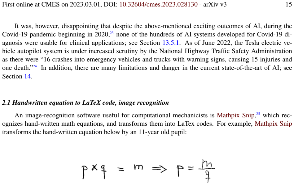
Figure 4. Figure 4: Handwritten equation 1 (Section 2.1) into this LaTeX code “p \times q = m \Rightarrow p = \frac { m } { q }” to yield the equation image: p × q = m ⇒ p = m q (1) Another example is the hand-written multiplication work below by the same pupil [PITH_FULL_IMAGE:figures/full_fig_p015_4.png] view at source ↗
Figure 5
Figure 5. Figure 5: Handwritten equation 2 (Section 2.1). Hand-written multiplication work of an eleven-year old pupil. 23“The World Health Organization declares COVID-19 a pandemic” on 2020 Mar 11, CDC Museum COVID-19 Timeline, Internet archive 2022.06.02. 24Krisher T., Teslas with Autopilot a step closer to recall after wrecks, Associated Press, 2022.06.10. 25We thank Kerem Uguz for informing the senior author LVQ about Mat… view at source ↗
Figure 6
Figure 6. Figure 6: Artificial intelligence and subfields (Section 2.2). Three classes of methods— Artificial Intelligence (AI), Machine Learning (ML), and Deep Learning (DL)—and their rela￾tionship, with an example of method in each class. A knowledge-base method is an AI method, but is neither a ML method, nor a DL method. Support Vector Machine and spiking computing are ML methods, and thus AI methods, but not a DL method.… view at source ↗
Figure 7
Figure 7. Figure 7: Feedforward neural network (Section 2.3.1). A feedforward neural network in [38], rotated clockwise by 90 degrees to compare to its equivalent in [PITH_FULL_IMAGE:figures/full_fig_p018_7.png] view at source ↗
Figure 8
Figure 8. Figure 8: Artificial neuron (Section 2.3.1). A neuron with its multiple inputs O p−1 i (which are outputs from the previous layer (p−1), and thus the variable name “O”), processing operations (multiply inputs with network weights w p−1 ji , sum weighted inputs, add bias θ p j , activation func￾tion f), and single output O p j [38]. See the equivalent [PITH_FULL_IMAGE:figures/full_fig_p019_8.png] view at source ↗
Figure 9
Figure 9. Figure 9: Cube and distorted cube elements (Section 2.3.1). Regular and distorted linear hexahedral elements [38]. (Figure reproduced with permission of the authors.) prescribed accuracy, and (2) corrections to the quadrature weights by trying one million randomly generated sets of correction factors, among which the best one was retained. While Application 1.1 used one fully-connected (Section 4.6.1) feedforward ne… view at source ↗
Figure 10
Figure 10. Figure 10: Distributions of error ratios defined by Eq. (21), when using correction factors estimated by deep learning. 3.5.2.3. Application phase [PITH_FULL_IMAGE:figures/full_fig_p020_10.png] view at source ↗
Figure 11
Figure 11. Figure 11: Dual-porosity single-permeability medium (Section 2.3.2). Left: Actual reservoir. Dual (or double) porosity indicates the presence of two types of porosity in naturally-fractured reservoirs (e.g., of oil): (1) Primary porosity in the matrix (e.g., voids in sands) with low per￾meability, within which fluid does not flow, (2) Secondary porosity due to fractures and vugs (cavities in rocks) with high (anisot… view at source ↗
Figure 12
Figure 12. Figure 12: Pore structure of Majella limestone, dual porosity (Section 2.3.2), a carbonate rock with high total porisity at 30%. Backscattered SEM images of Majella limestone: (a)- (c) sequence of zoomed-ins; (d) zoomed-out. (a) The larger macropores (dark areas) have dimensions comparable to the grains (allochems), having an average diameter of 54 µm, with macroporosity at 11.4%. (b) Micropores embedded in the grai… view at source ↗
Figure 13
Figure 13. Figure 13: Majella limestone, nonlinear stress-strain relations (Section 2.3.2). Differential stress (i.e., the difference between the largest principal stress and the smallest one) vs axial strain (left) and vs volumetric strain (right) [90]. See Remark 11.7, Section 11.3.4, and Re￾mark 11.10, Section 11.3.5. (Figure reproduced with permission of the authors.) non-linear stress-strain relationship can be related to… view at source ↗
Figure 7
Figure 7. Figure 7: Hierarchy of a multi-scale multi-physics poromechanics problem for fluid-infiltrating media. Black arrow represents a definition or a “universal principle”; red arrow represents either a phenomenological relation or an operator that is defined not based on first principles. (For interpretation of the references to color in this figure legend, the reader is referred to the web version of this article.) trai… view at source ↗
Figure 15
Figure 15. Figure 15: LSTM variant with “peephole” connections, block diagram (Sections 2.3.2, 7.2).43 Unlike the original LSTM unit (see Section 7.2), both the input gate and the forget gate in an LSTM unit with peephole connections receive the cell state as input. The above figure from Wikipedia, version 22:56, 4 October 2015, is identical to [PITH_FULL_IMAGE:figures/full_fig_p026_15.png] view at source ↗
Figure 16
Figure 16. Figure 16: Coordination number CN (Section 2.3.2, 11.3.2). (a) Chemistry. Number of bonds to the central atom. Uranium borohydride U(BH4)4 has CN = 12 hydrogen bonds to uranium. (b, c) Photoelastic discs showing number of contact points (coordination number) on a particle. (b) Random packing and force chains, different force directions along principal chains and in secondary particles. (c) Arches around large pores,… view at source ↗
Figure 17
Figure 17. Figure 17: Network with LSTM and microstructure data (porosity ϕ, coordination number CN = Nc, [PITH_FULL_IMAGE:figures/full_fig_p028_17.png] view at source ↗
Figure 18
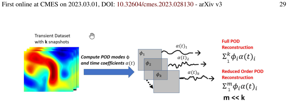
Figure 18. Figure 18: Reduced-order POD basis (Sections 2.3.3, 12.1). For each dataset (also Fig￾ure 116), which contained k snapshots, the full POD reconstruction of the flow-field dynamical quantity u(x, t), where x is a point in the 3-D flow field, consists of all k basis functions ϕi(x), with i = 1, . . . , k, using Eq. (3); see also Eq. (439). Typically, k is large; a reduced-order POD basis consists of selecting m ≪ k ba… view at source ↗
Figure 6
Figure 6. Figure 6: LSTM-ROM Methodology using the LSTM NN. An important assumption often made in ROM, including Galerkin-based ROM, is that the dominant POD modes for the training and test datasets are qualitatively similar [4]. For instance, flows within a narrow range of Reynolds number can exhibit qualitatively (but not quantitative) similar behavior, which are encoded in their dominant POD modes [4]. For the ISO training… view at source ↗
Figure 10
Figure 10. Figure 10: LSTM and BiLSTM predictions of Dominant POD ↵(t + t 0 ) for Isotropic turbulence test data [PITH_FULL_IMAGE:figures/full_fig_p031_10.png] view at source ↗
Figure 11
Figure 11. Figure 11: Mean Absolute Scaled Error (MASE) for LSTM predictions on all test samples in ISO dataset 5023 realizations. The results show that the MASE is generally low, except at samples where a sudden increase is observed. A similar trend is also observed for BiLSTM in [PITH_FULL_IMAGE:figures/full_fig_p031_11.png] view at source ↗
Figure 22
Figure 22. Figure 22: Function mapping, graphical representation (Section 4.3.1): n inputs in x ∈ R n×1 (n × 1 column matrix of real numbers) are fed into function f to produce m outputs in y ∈ R m×1 . The multiple levels of compositions in Eq. (18) can then be represented by x = y (0) | {z } Input f (1) −→ y (1) f (2) −→ · · · y (ℓ−1) f (ℓ) −→ y (ℓ) · · · f (L−1) −→ y (L−1) f (L) −→ | {z } Network as multilevel composition of… view at source ↗
Figure 23
Figure 23. Figure 23: Feedforward network (Sections 4.3.1, 4.4.4): Multilevel composition in feedfor￾ward network with L layers represented as a sequential application of functions f (ℓ) , with ℓ = 1, · · · , L, to n inputs gathered in x = y (0) ∈ R n×1 (n × 1 column matrix of real num￾bers) to produce m outputs gathered in y (L) = ye ∈ R m×1 . This figure is a higher-level block diagram that corresponds to the lower-level neu… view at source ↗
Figure 1.2
Figure 1.2. Figure 1.2: Figure1.2. See also Remark [PITH_FULL_IMAGE:figures/full_fig_p037_1_2.png] view at source ↗
Figure 24
Figure 24. Figure 24: Activation function (Section 4.4.2): Rectified linear function and its derivatives. See also Section 5.3.3 and [PITH_FULL_IMAGE:figures/full_fig_p040_24.png] view at source ↗
Figure 25
Figure 25. Figure 25: Current I versus voltage V (Section 4.4.2): Ideal diode, resistance, scaled rectified linear function as activation (transfer) function for the ideal diode and resistance in series. (Figure plotted with R = 2.) See also [PITH_FULL_IMAGE:figures/full_fig_p040_25.png] view at source ↗
Figure 26
Figure 26. Figure 26: Halfwave rectifier circuit (Section 4.4.2), with a primary alternative current z going in as input (left), passing through a transformer to lower the voltage amplitude, with the sec￾ondary alternative current out of the transformer being put through a closed circuit with an ideal diode D and a resistor R in series, resulting in a halfwave output current, which can be grossly approximated by the scaled rec… view at source ↗
Figure 27
Figure 27. Figure 27: FI curves (Sections 4.4.2, 13.2.2). Firing rate frequency (F) versus applied depo￾larizing current (I), thus FI curves. Three types of FI curves. The time histories of voltage Vm provide a visualization of the spikes, current threshold, and spike firing rates. The applied (input) current Iapp in increased gradually until it passes a current threshold, then the neuron begins to fire. Two input current leve… view at source ↗
Figure 28
Figure 28. Figure 28: FI or FV curves (Sections 3, 4.4.2, 13.2.2). Neuron firing rate (F) versus input current (I) (FI curves, a,b,c) or voltage (V). The Integrate-and-Fire model in SubFigure (c) can be used to replace the sigmoid function to fit the experimental data points in SubFigure (a). The ReLU function in [PITH_FULL_IMAGE:figures/full_fig_p043_28.png] view at source ↗
Figure 29
Figure 29. Figure 29: Halfwave rectifier (Sections 4.4.2, 5.3.2). Current I versus voltage V [red line in SubFigure (b)] in the halfwave rectifier circuit of [PITH_FULL_IMAGE:figures/full_fig_p044_29.png] view at source ↗
Figure 30
Figure 30. Figure 30: Logistic sigmoid function (Sections 4.4.2, 5.1.3, 5.3.1, 13.3.3): s(z) = [1 + exp(−z)]−1 = [tanh(z/2) + 1]/2 (red), with the tangent at the origin z = 0 (blue). See also Remark 5.3 and [PITH_FULL_IMAGE:figures/full_fig_p045_30.png] view at source ↗
Figure 31
Figure 31. Figure 31: Hyperbolic tangent function (Section 4.4.2): g(z) = tanh(z) = 2s(2z) − 1 (red) and its tangent g(z) = z at the coordinate origin (blue), showing that this activation function is identity for small signals. (2) Distributivity. Each feature of the data is represented distributively by many inputs, and each input is involved in distributively representing many features. Distributed representation is a key co… view at source ↗
Figure 32
Figure 32. Figure 32: One-layer network (Section 4.4.3) representing the relation between the predicted output ye and the input x, i.e., ye = f(x) = a(W x + b) = a(z), with the weighted sum z := W x + b; see Eq. (26) and Eq. (35) with ℓ = 1. For a lower-level details of this one layer, see [PITH_FULL_IMAGE:figures/full_fig_p045_32.png] view at source ↗
Figure 33
Figure 33. Figure 33: One-layer network (Section 4.4.3) in [PITH_FULL_IMAGE:figures/full_fig_p046_33.png] view at source ↗
Figure 35
Figure 35. Figure 35: Low-level details of layer (ℓ) (Sections 4.4.3, 4.4.4) of the multilayer neural net￾work in [PITH_FULL_IMAGE:figures/full_fig_p046_35.png] view at source ↗
Figure 36
Figure 36. Figure 36: Artificial neuron (Sections 2.3.1, 4.4.4, 13.1), row i in layer (ℓ) in [PITH_FULL_IMAGE:figures/full_fig_p046_36.png] view at source ↗
Figure 37
Figure 37. Figure 37: Representing XOR function (Sections 4.5, 13.2). This one-layer network (which is not the Rosenblatt perceptron in [PITH_FULL_IMAGE:figures/full_fig_p048_37.png] view at source ↗
Figure 38
Figure 38. Figure 38: Representing XOR function (Sections 4.5). This two-layer network can perform this task. The four points in the design matrix X = [x1, . . . , x4] ∈ R 2×4 (see [PITH_FULL_IMAGE:figures/full_fig_p049_38.png] view at source ↗
Figure 39
Figure 39. Figure 39: Two-layer network for XOR representation (Sections 4.5). Left: XOR function, with A = x (1) 1 = [0, 0]T , B = x (1) 2 = [0, 1]T , C = x (1) 3 = [1, 0]T , D = x (1) 4 = [1, 1]T ; see Eq. (52). The XOR value for the solid red dots is 1, and for the open blue dots 0. Right: Images of points A, B, C, D in the z-plane due only to the first term of Eq. (54), i.e., w(1)X(1), which is shown in Eq. (55). See also … view at source ↗
Figure 40
Figure 40. Figure 40: Two-layer network for XOR representation (Sections 4.5). Left: Images of points A, B, C, D of Z(1) in Eq. (56), obtained after a translation by adding the bias b (1) = [0, −1]T in Eq. (51) to the same points A, B, C, D in the right subfigure of [PITH_FULL_IMAGE:figures/full_fig_p051_40.png] view at source ↗
Figure 41
Figure 41. Figure 41: Test accuracy versus network depth (Section 4.6.1), showing that test accuracy for this example increases monotonically with the network depth (number of layers). [78], p. 196. (Figure reproduced with permission of the authors.) But it is not clear where in [13] that it was actually said that a network is “deep” if the number of hidden (state) layers is greater than three. An example in image recognition … view at source ↗
Figure 42
Figure 42. Figure 42: Increasing network size over time (Section 4.6.1, 13.2). All networks before 2015 had their number of neurons smaller than that of a frog at 1.6 × 10⁷ , and still far below that in a human brain at 8.6 × 10¹⁰; see “List of animals by number of neurons”, Wikipedia, version 02:46, 9 May 2019. In [78], p. 23, it was estimated that neural network size would double every 2.4 years (a clear parallel to Moore’s … view at source ↗
Figure 43
Figure 43. Figure 43: Training/test error vs. iterations, depth (Sections 4.6.2, 6). The training error and test error of deep fully-connected networks increased when the number of layers (depth) increased [127]. (Figure reproduced with permission of the authors.) [PITH_FULL_IMAGE:figures/full_fig_p056_43.png] view at source ↗
Figure 44
Figure 44. Figure 44: Residual network (Sections 4.6.2, 6), basic building block having two layers with the rectified linear activation function (ReLU), for which the input is x, the output is H(x) = F(x) + x, where the internal mapping function F(x) = H(x) − x is called the residual. Chaining this building block one after another forms a deep residual network; see [PITH_FULL_IMAGE:figures/full_fig_p056_44.png] view at source ↗
Figure 45
Figure 45. Figure 45: Full residual network (Sections 4.6.2, 6) with 34 layers, made up from 16 building blocks with two layers each ( [PITH_FULL_IMAGE:figures/full_fig_p057_45.png] view at source ↗
Figure 46
Figure 46. Figure 46: Sofmax function for two classes, logistic sigmoid (Section 5.1.3, 5.3.1): s(z) = [1 + exp(−z)]−1 and s(−z) = [1 + exp(z)]−1 , such that s(z) + s(−z) = 17. See also [PITH_FULL_IMAGE:figures/full_fig_p061_46.png] view at source ↗
Figure 47
Figure 47. Figure 47: Backpropagation building block, typical layer (ℓ) (Section 5.2, Algorithm 1, Ap￾pendix 1). The forward propagation path is shown in blue, with the backpropagation path in red. The update of the parameters θ (ℓ) in layer (ℓ) is done as soon as the gradient ∂J/∂θ (ℓ) is available using a gradient descent algorithm. The row matrix r (ℓ) = ∂J/∂z (ℓ) in Eq. (104) can be computed once for use to evaluate both t… view at source ↗
Figure 48
Figure 48. Figure 48: Backpropagation in fully-connected network (Section 5.2, 5.3, Algorithm 1, Ap￾pendix 1). Starting from the predicted output ye = y (L) In the last layer (L) at the end of any forward propagation (blue arrows), and going backward (red arrows) to the first layer with ℓ = L, · · · , 1, and along the way at layer (ℓ), compute the gradient of the cost function J relative the the parameters θ (ℓ) to update thos… view at source ↗
Figure 49
Figure 49. Figure 49: Vanishing gradient problem (Section 5.3). Speed of learning of earlier layers is much slower than that of later layers. Here, after 400 epochs of training, the speed of learning of Layer (1) at 10−5 (blue line) is 100 times slower than that of Layer (4) at 10−3 (green line); [21], Chapter 5, ‘Why are deep neural networks hard to train ?’ (CC BY-NC 3.0). To understand the reason for the quick and significa… view at source ↗
Figure 50
Figure 50. Figure 50: Neural network with four layers (Section 5.3), one neuron per layer, scalar input x, scalar output y, cost function J(θ) = 1 2 (y − ye) 2 , with ye = y (4) being the target output and also the output of layer (4), such that f (ℓ) (y (ℓ−1)) = a(z (ℓ) ), with a(·) being the active function, z (ℓ) = w (ℓ)y (ℓ−1) + b (ℓ) , for ℓ = 1, . . . , 4, and the network parameters are θ = [w1, . . . , w4, b1, . . . , b… view at source ↗
Figure 51
Figure 51. Figure 51: Neural network with four layers in [PITH_FULL_IMAGE:figures/full_fig_p068_51.png] view at source ↗
Figure 52
Figure 52. Figure 52: Successive multiplications of these derivatives will result in smaller and smaller values along the back propagation path. If the weights w (ℓ) in Eq. (110) are also smaller than 1, then the gradient ∂J/∂b(1) will tend toward 0, i.e., vanish. The problem is further exacerbated in deeper networks with increasing number of layers, and thus increasing number of factors less than 1 (i.e., |a ′ (z (ℓ) )w (ℓ) )… view at source ↗
Figure 53
Figure 53. Figure 53: Cost-function cliff (Section 5.3.1). A cliff, or a sharp drop in the cost function. The parameter space is represented by a weight w and a bias b. The slope at the brink of the cliff leads to large-magnitude gradients, which when multiplied with each other several times along the back propagation path would result in an exploding gradient problem. [78], p. 281. (Figure reproduced with permission of the au… view at source ↗
Figure 54
Figure 54. Figure 54: Rectified Linear Unit (ReLU, left) and Parametric ReLU (right) (Section 5.3.2), in which the slope s is a parameter to optimize; see Section 5.3.3. See also [PITH_FULL_IMAGE:figures/full_fig_p071_54.png] view at source ↗
Figure 55
Figure 55. Figure 55: Cost-function landscape (Section 6). Residual network with 56 layers (ResNet-56) on the CIFAR-10 training set. Highly non-convex, with many local minima, and deep, narrow valleys [132]. The training error and test error for fully-connected network increased when the number of layers was increased from 20 to 56, [PITH_FULL_IMAGE:figures/full_fig_p071_55.png] view at source ↗
Figure 56
Figure 56. Figure 56: Training set, validation set, test set (Section 6.1). Partition of whole dataset. The examples are independent. The three subsets are identically distributed. 6.1 Training set, validation set, test set, stopping criteria The classical (old) thinking—starting in 1992 with [133] and exemplified by Figures 57, 58, 59, 60 (a, left)—would surprise first-time learners that minimizing the training error is not o… view at source ↗
Figure 57
Figure 57. Figure 57: Training and validation learning curves—Classical viewpoint (Section 6.1), i.e., plots of training error and validation errors versus epoch number (time). While the training cost decreased continuously, the validation cost reaches a minimum around epoch 20, then started to gradually increase, forming an “asymmetric U-shaped curve.” Between epoch 100 and epoch 240, the training error was essentially flat, … view at source ↗
Figure 58
Figure 58. Figure 58: Validation learning curve (Section 6.1, Algorithm 4). Validation error vs epoch number. Some validation error could oscillate wildly around the mean, resulting in an “ugly reality”. The global minimum validation error corresponded to epoch number τ ⋆ . Since the stopping criteria may miss this global minimum, it was suggested to monitor the validation learning curve to find the epoch τ ⋆ at which the netw… view at source ↗
Figure 59
Figure 59. Figure 59: Bias-variance trade-off (Section 6.1). Training error (cost) and test error versus model capacity. Two ways to change the model capacity: (1) change the number of network parameters, (2) change the values of these parameters (weight decay). The generalization gap is the difference between the test (generalization) error and the training error. As the model capacity increases from underfit to overfit, the … view at source ↗
Figure 60
Figure 60. Figure 60: Modern interpolation regime (Sections 6.1, 14.2). Beyond the interpolation thresh￾old, the test error goes down as the model capacity (e.g., number of parameters) increases, describing the observation that networks with high capacity beyond the interpolation threshold generalize well, even though overfit in training. Risk = error or cost. Capacity = number of parameters (but could also be increased by wei… view at source ↗
Figure 61
Figure 61. Figure 61: Empirical test error vs Number of paramesters (Sections 6.1, 14.2). Experiments using the MNIST handwritten digit database in [137] confirmed the modern interpolation regime in [PITH_FULL_IMAGE:figures/full_fig_p077_61.png] view at source ↗
Figure 62
Figure 62. Figure 62: Inexact line search, Goldstein’s rule (Section 6.2.4). acceptable step lengths would be such that a decrease in the cost function J, denoted by ∆J in Eq. (124), falls into an acceptable sector formed by an upper-bound line and a lower-bound line. the upper bound is given by the straight line α ϵ g• d (green), with fixed constant α ∈ (0, 1 2 ) and ϵ g• d < 0 being the slope to the curve ∆J(ϵ) at ϵ = 0. The… view at source ↗
Figure 63
Figure 63. Figure 63: SGD with momentum, small heavy sphere Section 6.3.2. The descent direction (negative gradient, black arrows) bounces back and forth between the steep slopes of a deep and narrow valley. The small-heavy-sphere method, or SGD with momentum, follows a faster descent (red path) toward the bottom of the valley. See the cost-function landscape with deep valleys in [PITH_FULL_IMAGE:figures/full_fig_p089_63.png] view at source ↗
Figure 64
Figure 64. Figure 64: Optimal minibatch size vs. training-set size (Section 6.3.5). For a given training￾set size, the smallest minibatch size that achieves the highest accuracy is optimal. Left figure: The optimal mimibatch size was moving to the right with increasing training-set size M. Right figure: The optimal minibatch size in [186] is linearly proportional to the training-set size M for large training sets (i.e., M → ∞)… view at source ↗
Figure 65
Figure 65. Figure 65: Minibatch-size increase vs. step-length decay, training schedules (Section 6.3.5). Left figure: Step length (learning rate) vs. number of epochs. Right figure: Minibatch size vs. number of epochs. Three learning-rate schedules167 were used for training: (1) The step length was decayed by a factor of 5, from an initial value of 10−1 , at specific epochs (60, 120, 160), while the minibatch size was kept con… view at source ↗
Figure 66
Figure 66. Figure 66: Minibatch-size increase, fewer parameter updates, faster comutation (Sec￾tion 6.3.5). For each of the three training schedules in [PITH_FULL_IMAGE:figures/full_fig_p098_66.png] view at source ↗
Figure 67
Figure 67. Figure 67: Weight decay (Section 6.3.6). Effects of magnitude of weight-decay parameter d. Adapted from [78], p. 116. (Figure reproduced with permission of the authors.) 6.3.7 Combining all add-on tricks To have a general parameter-update equation that combines all of the above add-on improvement tricks, start with the parameter update with momentum and accelerated gradient Eq. (141) θe k+1 = θe k − ϵkge(θe k + γk(θ… view at source ↗
Figure 68
Figure 68. Figure 68: Convergence of adaptive learning-rate algorithms (Section 6.3.2): AdaGrad, RM￾SProp, SGDNesterov, AdaDelta, Adam [170]. (Figure reproduced with permission of the authors.) 6.5.2 AdaGrad: Adaptive Gradient Starting the line of research on adaptive learning-rate algorithms, the authors of [52] 182 selected the following functions for Algorithm 5: ϕk(ge1, . . . , gek) = gek , with χϕk = I (Identity) ⇒ mk = g… view at source ↗
Figure 69
Figure 69. Figure 69: Dow Jones Industrial Average (DJIA, Section 6.5.3) stock index year-to-date (YTD) chart as from 2019.01.01 to 2019.11.30, Google Finance. “Exponential smoothing methods have been around since the 1950s, and are still the most popular fore￾casting methods used in business and industry” such as “minute-by-minute stock prices, hourly temperatures at a weather station, daily numbers of arrivals at a medical c… view at source ↗
Figure 70
Figure 70. Figure 70: Saudi Arabia oil production during 1996-2013 (Section 6.5.3). Piecewise linear data (black) and fitted curve (red), despite the name “smoothing”. From [207], Chap. 7. (Figure reproduced with permission of the authors.) For neural networks, early use of exponential smoothing dates back at least to 1998 in [165] and [166].185 For adaptive learning-rate algorithms further below (RMSProp, AdaDelta, Adam, etc.… view at source ↗
Figure 71
Figure 71. Figure 71: AMSGrad vs Adam, numerical examples (Sections 6.1, 6.5.7). The MNIST dataset is used. The first two figures on the left were the results of using logistic regression (network with one layer with logistic sigmoid activation function), whereas the figure on the right is by using a neural network with three layers (input layer, hidden layer, output layer). The cost function decreased faster for AMSGrad compa… view at source ↗
Figure 72
Figure 72. Figure 72: Overfitting (Section 6.5.9, 6.5.10). Left: Underfitting with 1st-order polynomial. Middle: Appropriate fitting with 2nd-order polynomial. Right: Overfitting with 9th-order poly￾nomial. See [78], p. 110, Figure5.2. (Figure reproduced with permission of the authors.) 6.5.9 Criticism of adaptive methods, resurgence of SGD Yet, despite the claim that RMSProp is “currently one of the go-to optimization methods… view at source ↗
Figure 73
Figure 73. Figure 73: Standard SGD and SGD with momentum vs AdaGrad, RMSProp, Adam on CIFAR￾10 dataset (Sections 6.1, 6.3.2, 6.5.9). From [55], where a method for step-size tuning and step-size decaying was proposed to achieve lowest training error and generalization (test) error for both Standard SGD and SGD with momentum (“Heavy Ball” or better yet “Small Heavy Sphere” method) compared to adaptive methods such as AdaGrad, RM… view at source ↗
Figure 74
Figure 74. Figure 74: AdamW vs Adam, SGD, and variants on CIFAR-10 dataset (Sections 6.1, 6.5.10). While AdamW achieved lowest training loss (error) after 1800 epochs, the results showed that SGD with weight decay (SGDW) and with warm restart (SGDWR) achieved lower test (generalization) errors than Adam, AdamW, AdamWR. See [PITH_FULL_IMAGE:figures/full_fig_p116_74.png] view at source ↗
Figure 75
Figure 75. Figure 75: Cosine annealing (Sections 6.3.4, 6.5.10). Annealing factor ak as a function of epoch number. Four annealing cycles p = 1, . . . , 4, with the following schedule for Tp in Eq. (154): (1) Cycle 1, T1 = 100 epochs, epoch 0 to epoch 100, (2) Cycle 2, T2 = 200 epochs, epoch 101 to epoch 300, (3) Cycle 3, T3 = 400 epochs, epoch 301 to epoch 700, (4) Cycle 4, T4 = 800 epochs, epoch 701 to epoch 1500. From [56].… view at source ↗
Figure 76
Figure 76. Figure 76: CIFAR-100 test loss using Resnet-34 and DenseNet-121 (Section 6.5.10). Compar￾ison between various optimizers, including Adam and AdamW, showing that SGD achieved the lowest global minimum loss (blue line) compared to all adaptive methods tested as shown [168]. See also [PITH_FULL_IMAGE:figures/full_fig_p118_76.png] view at source ↗
Figure 77
Figure 77. Figure 77: SGD frequently outperformed all adaptive methods (Section 6.5.10). The table contains the global minimum for each optimizer, for each of the two datasets CIFAR-10 and CIFAR-100, using two different networks. For each network, an error percentage and the loss (cost) were given. Shown in red are the lowest global minima obtained by SGD in the corresponding columns. Even in the three columns in which SGD res… view at source ↗
Figure 78
Figure 78. Figure 78: Stochastic Newton with Armijo-like 2nd order line search (Section 6.7). IJCNN1 dataset from the LIBSVM library. Three batch sizes were used (1%, 5%, 100%) for both SGD and ALAS (stochastic Newton Algorithm 7). The exact gradient norm for each of these six cases was plotted against the training epochs on the left, and against the iteration numbers on the right. An epoch is the number of non-overlapping min… view at source ↗
Figure 79
Figure 79. Figure 79: Folded and unfolded discrete RNN (Section 7.1, 13.2.2). Left: Folded discrete RNN at configuration (or state) number [k], where k is an integer, with input x [k] to a multilayer neural network f(·) = f (1) ◦ f (2) ◦ · · · ◦ f (L) (·) as in Eq. (18), having a feedback loop h [k−1] with delay by one step, to produce output h [k] . Right: Unfolded discrete RNN, where the feedback loop is unfolded, centered a… view at source ↗
Figure 80
Figure 80. Figure 80: RNN with two multilayer neural networks (MLNs), (Section 7.1) denoted by f1(·) and f2(·), whose outputs are fed into the loss function for optimization. This RNN is a gener￾alization of the RNN in [PITH_FULL_IMAGE:figures/full_fig_p128_80.png] view at source ↗
Figure 81
Figure 81. Figure 81: Folded Recurrent Neural Network (RNN) with Long Short-Term Memory (LSTM) cell (Section 7.2, 11.3.3). The cell state at [k] is denoted by z [k] s ≡ c [k] . Two feedback loops, one for cell state zs and one for hidden state h, with one-step delay [k − 1]. The key unified recurring relation is Fα = Aα(z [k] α ), with α ∈ {s (state), f (forget), I (Input), g (external input), O (Output)}, where Aα is a sigmoi… view at source ↗
Figure 82
Figure 82. Figure 82: Unfolded RNN with LSTM cells (Sections 2.3.2, 7.2, 12.1): In this unfolded RNN, the cell states are centered at the LSTM cell [k = n], preceded by the LSTM cell [k = n − 1], and followed by the LSTM cell [k = n+ 1]. See Eq. (290) for the recurring relation among the successive cell states, and [PITH_FULL_IMAGE:figures/full_fig_p132_82.png] view at source ↗
Figure 83
Figure 83. Figure 83: Folded RNN with Gated Recurrent Unit (GRU) (Section 7.3). The cell state at [k − 1], i.e., (x [k−1] , h [k−1]) are inputs to produce the hidden state h [k] . One feedback loop for the hidden state h, with one-step delay [k − 1]. The key unified recurring relation is Fα = Aα(z [k−1] α ), with α ∈ {r (reset), u (update), O (Output)}, where Aα is a logistic sigmoi activation function, and z [k−1] α is a line… view at source ↗
Figure 84
Figure 84. Figure 84: Scaled dot-product attention and multi-head attention (Section 7.4.3). Scaled-dot product attention (left) is the elementary building block of the Transformer model. It compares query vectors (Q) against a set of key vectors (K) to produce a context vector by weighting to value vectors (V) that correspond to the keys. For this purpose, softmax(·) function is applied to the inner product (MatMul) of the qu… view at source ↗
Figure 85
Figure 85. Figure 85: Transformer architecture (Section 7.4.3). The Transformer is a sequence-to￾sequence model without recurrent connections. Encoder and decoder are entirely built upon scaled dot-product attention. Items of source and target sequences are numerically represented as vectors, i.e., embeddings. Positional encodings furnish embeddings with information on their positions within the respective sequences. The encod… view at source ↗
Figure 86
Figure 86. Figure 86: Gaussian process priors (Section 8.3). Left: Two samples with Gaussian kernel. Right: Two samples with Laplacian kernel. Parameters for both kernels: Kernel precision (inverse of variance) γ = σ −2 = 0.2 in Eq. (358), isotropic noise variance ν 2I = 10−6I added to covariance matrix Cyy of output y and isotropic weight covariance matrix Cww = Σ = I in Eq. (374). symmetry, we take it to be zero” [130], p. 3… view at source ↗
Figure 87
Figure 87. Figure 87: Gaussian process prior and posterior samplings, Gaussian kernel (Section 8.3). Top left: Gaussian-prior samples (Section 8.3.1). The shaded red zones represent the predic￾tive density of at each input location. Top right: Gaussian-posterior samples with 1 data point. Bottom left: Gaussian-posterior samples with 2 data points. Bottom right: Gaussian-posterior samples with 3 data points [247]. See [PITH_FU… view at source ↗
Figure 88
Figure 88. Figure 88: Gaussian process posterior samplings, noise effects (Section 8.3). Not all sampled curves in [PITH_FULL_IMAGE:figures/full_fig_p152_88.png] view at source ↗
Figure 89
Figure 89. Figure 89: Gaussian process posterior samplings, animation (Section 8.3). Interactive Gaus￾sian Process Visualization, Infinite curiosity. Click on the plot area to specify data points. See Figures 87 and 88. DL-related software framework, see [PITH_FULL_IMAGE:figures/full_fig_p153_89.png] view at source ↗
Figure 90
Figure 90. Figure 90: Top deep-learning libraries in 2018 by the “Power Score” in [249]. By 2022, using Google Trends, the popularity of different frameworks is significantly different; see [PITH_FULL_IMAGE:figures/full_fig_p154_90.png] view at source ↗
Figure 91
Figure 91. Figure 91: Google Trends of deep-learning software libraries (Section 9). The chart shows the popularity of five DL-related software libraries most “powerful” in 2018 over the last 5 years (as of July 2022). See also [PITH_FULL_IMAGE:figures/full_fig_p155_91.png] view at source ↗
Figure 92
Figure 92. Figure 92: Positioning and pointing control of large deformable beam (Section 9, Remark 9.1). Reinforcement learning. The agent is trained to align the tip of the flexible beam with the target position (red ball). For this purpose, the agent can move the base of the cantilever; the environment returns the negative Euclidean distance of the beam’s tip to the target position as “reward” in each time-step of the simula… view at source ↗
Figure 93
Figure 93. Figure 93: DL-frameworks in nonlinear finite-element problems (Section 9.4). The computa￾tional efficiency of a PyTorch-based (Version 1.8) finite-element code implemented was com￾pared against the state-of-the-art general purpose Netgen/NGSolve [265] for a problem of non￾linear elasticity, see the slides of the presentation and the corresponding video. The figures show timings (in seconds) for evaluations of the st… view at source ↗
Figure 94
Figure 94. Figure 94: Physics-Informed Neural Networks (PINN) concept (Section 9.5). The goal is to find the optimal network parameters θ ⋆ (weights) and PDE parameters λ ⋆ that minimize the total weighted loss function L(θ, λ), which is a linear combination of four loss functions: (1) The residual of the PDE, LPDE, (2) Loss due to initial conditions, LIC, (3) Loss due to boundary conditions , LBC, (4) Loss due to known (label… view at source ↗
Figure 95
Figure 95. Figure 95: Coupled nonlinear hyperbolic equations (Section 9.5). Analytical solution, pre￾dicted solution by NeuralPDE [275] and error for the coupled nonlinear hyperbolic equations in Eq. (383). Additional PINN software packages other than those in [PITH_FULL_IMAGE:figures/full_fig_p160_95.png] view at source ↗
Figure 7
Figure 7. Figure 7: Nodes A, B and D of any 8-noded element are shifted to x-y plane by translation (a) and rotations (b), (c) and (d). E (±rd, ±rd, 1 ± rd), F (1 ± rd, ±rd, 1 ± rd), G (1 ± rd, 1 ± rd, 1 ± rd), and H (±rd, 1 ± rd, 1 ± rd). Here, the maximum amount of change in the coordinate values is selected from d = 0.1, 0.2, 0.3, 0.4 and 0.5. It is noted that, if the coordinates of each node in an element are independentl… view at source ↗
Figure 97
Figure 97. Figure 97: Creation of randomly distorted elements (Section 10). Hexahedra forming the train￾ing and validation sets are created by randomly displacing the nodes of a regular hexahedral. To comply with the normalization procedure, node A remains fixed, node B is shifted along the x-axis and node C is displaced with the xy-plane. For each of the remaining nodes (E, F, G, H), all three nodal coordinates are varied ran… view at source ↗
Figure 98
Figure 98. Figure 98: Method 1, Optimal number of integration points, feasibility (Section 10.2.1). Dis￾tribution of minimum numbers of integration points on a local coordinate axes for a maximum error of e tol = 10−3 among 10,000 elements generated randomly using the method in Fig￾ure 97. For d = 0.1, all elements were only slightly distorted, and required 3 integration points each. For d = 0.5, close to 5,000 elements requir… view at source ↗
Figure 99
Figure 99. Figure 99: Method 1, Optimal network architecture for training (Section 10.2.2). The number of hidden layers varies from 1 to 5, keeping the number of neurons per hidden layer constant at 50. The network with 3 hidden layers provided the highest accuracy for both the training set (“patterns”) at 98.6% and for the validation set (“test patterns”) at 81.6%. Increase the network depth does not necessarily increase the … view at source ↗
Figure 100
Figure 100. Figure 100: Method 1, application phase (Section 10.2.3). The numbers of quadrature points predicted by the neural network was compared to the minimum numbers of quadrature points for maximum error e tol = 10−3 [38]. Table (a) shows the results for the training set (“pat￾terns”), and Table (b) for the validation set. (Table reproduced with permission of the authors.) i.e., {w opt i,j,k} = arg min wi,j,k Rerror, (403… view at source ↗
Figure 101
Figure 101. Figure 101: Method 2, Quadrature weight correction, feasibility (Section 10.3.1). Each ele￾ment was tested 1 million times with randomly generated sets of quadrature weights. There were 4000 elements in each of the 5 groups with different degrees of maximum distortion, d. Quadrature weight correction effectiveness increased with element distortion. Weakly distorted elements (d = 0.1) did not have any improvement, an… view at source ↗
Figure 102
Figure 102. Figure 102: Method 2, training phase, classifier network (Section 10.3.2). The training and validation sets comprised 5000 elements each, of which 3707 and 3682, respectively, belonged to Category A (no improvements upon weight correction). A first neural network with 4 hidden layers of 30 neurons correctly classified (3707 + 1194)/5000 ≈ 98 % elements in the training set (a) and (3682 + 939)/5000 ≈ 92 % elements in… view at source ↗
Figure 103
Figure 103. Figure 103: Method 2, training phase, regression network (Section 10.3.2). A second neu￾ral network estimated 8 correction factors {wi,j,k}, with i, j, k ∈ {1, 2}, to be multiplied by the standard quadrature weights for each element. Distribution of normalized errors, i.e., the normalized differences between the predicted weights (outputs) Oj and the true weights Tj for the elements of the training set (red) and the… view at source ↗
Figure 10
Figure 10. Figure 10: Distributions of error ratios defined by Eq. (21), when using correction factors estimated by deep learning. to deduce the constitutive behavior on the macroscopic scale is evaluated at the quadrature points of the [PITH_FULL_IMAGE:figures/full_fig_p172_10.png] view at source ↗
Figure 104
Figure 104. Figure 104: Three scales in data-driven fault-reactivation simulations (Sections 2.3.2, 11.1, 11.3.5). Relative orientation of Representative Volume Elements (RVEs). Left: Microscale (µ) RVE using Discrete Element Method (DEM), [PITH_FULL_IMAGE:figures/full_fig_p173_104.png] view at source ↗
Figure 105
Figure 105. Figure 105: Single-physics block diagram (Section 11.2). Single physics is an easiest way to see the role of deep learning in modeling complex nonlinear constitutive behavior (stress￾strain relation, red arrow), as first realized in [23], where balance of linear momentum and strain-displacement relation are definitions or accepted “universal principles” (black arrows) [25] (Figure reproduced with permission of the a… view at source ↗
Figure 106
Figure 106. Figure 106: Microscale RVE (Sections 11.3.2, 11.3.3, 11.3.5). A 10 cm × 10 cm × 5 cm box of identical spheres of 0.5 cm diameter ( [PITH_FULL_IMAGE:figures/full_fig_p175_106.png] view at source ↗
Figure 107
Figure 107. Figure 107: Optimal RNN-LSTM architecture (Section 11.3.3). 5 different configurations of RNNs with LSTM units [25]. (Table reproduced with permission of the authors.) 11.3.3 Optimal RNN-LSTM architecture Using the same discrete element assembly of microscale RVE in [PITH_FULL_IMAGE:figures/full_fig_p175_107.png] view at source ↗
Figure 108
Figure 108. Figure 108: Optimal RNN-LSTM architecture (Section 11.3.3). Training error and test errors for 5 different configurations of RNN with LSTM units, see [PITH_FULL_IMAGE:figures/full_fig_p176_108.png] view at source ↗
Figure 109
Figure 109. Figure 109: Optimal RNN-LSTM architecture (Section 11.3.3). Training error (a) and testing error (b), close-up views of [PITH_FULL_IMAGE:figures/full_fig_p177_109.png] view at source ↗
Figure 110
Figure 110. Figure 110: Mesoscale RNN with LSTM units. Traction-separation law (Sections 11.3.3, 11.3.5). Left: Sequence of imposed displacement jumps on microscale RVE ( [PITH_FULL_IMAGE:figures/full_fig_p178_110.png] view at source ↗
Figure 111
Figure 111. Figure 111: Continuum with embedded strong discontinuity (Section 11.3.5). Domain B = B + ∪ B− with embedded discontinuity surface Γ, running through the middle of a narrow band (light blue) Bh = (B + h ∪ B− h ) ⊂ B between the parallel surfaces Γ + and Γ −. Objects behind Γ in the negative direction of the normal n to Γ are designated with the minus sign, and those in front of Γ with the plus sign. The narrow band … view at source ↗
Figure 112
Figure 112. Figure 112: Mesoscale RVE (Sections 11.3.3, 11.3.5). A 2-D domain of size 1 m × 1 m (Re￾mark 11.9). See [PITH_FULL_IMAGE:figures/full_fig_p180_112.png] view at source ↗
Figure 113
Figure 113. Figure 113: Mesoscale RVE (Section 11.3.3). Strains and displacement jumps [25] (Figure reproduced with permission of the authors.) where τ is the shear stress along the fault line, τp the critical shear stress for the onset of fault reactivation, C the cohesion strength, µ the coefficient of friction, σ ′ the effective stress normal to the fault line, σ the normal stress, and p the fluid pore pressure. The authors … view at source ↗
Figure 114
Figure 114. Figure 114: Mesoscale RVE (Section 11.3.5). Validation of coupled FEM and RNN with LSTM units (FEM-LSTM, red dotted line) against coupled FEM and DEM (FEM-DEM, blue line) to analyze the mesoscale RVE in [PITH_FULL_IMAGE:figures/full_fig_p182_114.png] view at source ↗
Figure 26
Figure 26. Figure 26: Loading path of three selected training cases TR1, TR2, TR3 and three selected testing cases TE1, TE2, TE3 on the meso-scale RVE. un and us are the normal and tangential displacement jumps. The coordinate system is {M, N} (or {x, y}) depicted in [PITH_FULL_IMAGE:figures/full_fig_p182_26.png] view at source ↗
Figure 115
Figure 115. Figure 115: Macroscale RNN with LSTM units (Section 11.3.5). Normal traction (Tn) vs im￾posed displacement jumps (Un) on mesoscale RVE ( [PITH_FULL_IMAGE:figures/full_fig_p183_115.png] view at source ↗
Figure 28
Figure 28. Figure 28: Comparison of the meso-scale FEM–LSTM simulation data and the trained macro-scale data-driven model. Tangential traction against tangential displacement jump for the selected training and testing cases. The numbers mark the sequence of loading–unloading cycles. MSE refers to the scaled mean squared error defined in Eq. (59) [PITH_FULL_IMAGE:figures/full_fig_p183_28.png] view at source ↗
Figure 116
Figure 116. Figure 116: 2-D datasets for training neural networks (Sections 2.3.3, 12.1). Extract 2-D datasets from 3-D turbulent flow field evolving in time. From the 3-D flow field, extract N equidistant 2-D planes (slices). Within each 2-D plane, select a region (yellow square), and k temporal snapshots of this region as it evolves in time to produce a dataset. Among these N datasets, each containing k snapshots of the same … view at source ↗
Figure 117
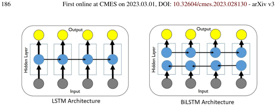
Figure 117. Figure 117: LSTM unit and BiLSTM unit (Sections 2.3.2, 2.3.3, 7.2, 12.2). Each blue dot is an original LSTM unit (in folded form [PITH_FULL_IMAGE:figures/full_fig_p186_117.png] view at source ↗
Figure 118
Figure 118. Figure 118: LSTM/BiLSTM training strategy (Sections 12.2.1, 12.2.2). From the 1-D time series αi(t) of each dominant mode ϕi , for i = 1, . . . , m, use a moving window to extract thousands of samples αi(t), t ∈ [tk, tspl k ], with tk being the time of snapshot k. Each sample is subdivided into an input signal αi(t), t ∈ [tk, tk + tinp] and an output signal αi(t), t ∈ [tk + tinp, tspl k ], with t spl k − tk = tinp +… view at source ↗
Figure 15
Figure 15. Figure 15: Training of a unified NN model for all POD dominant modes chaotic systems, they are outside the scope of this work. 4.2 Magnetohydrodynamic Turbulence The strategy in the previous section required a NN model to be trained for each POD mode - a multiple model approach. This approach implies that the NN learns universal features for the same mode between the various training datasets. The implicit assumptio… view at source ↗
Figure 120
Figure 120. Figure 120: Hurst exponent vs POD-mode rank for Isotropic Turbulence (ISO) (Sections 12.3). POD modes with larger eigenvalues (Eq. (438)) are higher ranked, and have lower rank number, e.g., POD mode rank 7 has larger eigenvalue, and thus more dominant, than POD mode rank 50. The Hurst exponent, even though fluctuating, trends downward with the POD mode rank, but not monotonically, i.e., for two POD modes sufficient… view at source ↗
Figure 121
Figure 121. Figure 121: Space-time solution of inviscid 1D-Burgers’ equation (Section 12.4.1). The solu￾tion shows a characteristic steep spatial gradient, which shifts and further steepens in the course of time. The FOM solution (left) and the solution of the proposed hyper-reduced ROM (center), in which the solution subspace is represented by a nonlinear manifold in the form of a feed￾forward neural network (Section 4) (NM-LS… view at source ↗
Figure 122
Figure 122. Figure 122: Dense vs. shallow decoder networks (Section 12.4.3). Contributing neurons (or￾ange “nodes”) and connections (orange “edges”) lie in the “active” paths arriving at the selected outputs (solid orange “nodes”) from the decoder’s inputs. In dense networks as the one in (a), each neuron in a layer is connected to all other neurons in both the preceeding layer (if it exists) and in the succeeding layer (if it … view at source ↗
Figure 123
Figure 123. Figure 123: Sparsity masks (Section 12.4.3) used to realize sparse decoders in one- and two￾dimensional problems. The structure of the respective binary-valued mask matrices S is in￾spired by grid-points required in the finite-difference approximation of the Laplace operator in one and two dimensions, respectively. (Figure reproduced with permission of the authors.) Using our notation for feedforward networks and ac… view at source ↗
Figure 124
Figure 124. Figure 124: Subnet construction (Section 12.4.4). To reduce computational cost, a subnet representing the set of active paths, which comprise all neurons and connections needed for the evaluation of selected outputs (highlighted in orange), i.e., the reduced residual rb, is con￾structed (left). The size of the hidden layer of the subnet depends on which output components of the decoder are needed for the reconstruct… view at source ↗
Figure 125
Figure 125. Figure 125: 2-D Burger’s equation. Solution snapshots of full and reduced-order models (Section 12.4.5). From left to right, the components u (top row) and v (bottom row) of the ve￾locity field at time t = 2 are shown for the FOM, the hyper-reduced nonlinear-manifold-based ROM (NM-LSPG-HR) and the hyper-reduced linear-subspace-based ROM (LS-LSPG-HR). Both ROMs have a dimension of ns = 5; with respect to hyper-reduct… view at source ↗
Figure 126
Figure 126. Figure 126: 2-D Burger’s equation. Reynolds number vs. singular values (Section 12.4.5). Performing SVD on FOM solution snapshots, which were partitioned into x and y-components, the influence of the Reynolds number on the singular values is illustrated. In diffusion￾dominated problems, which are characterized by low Reynolds number, a rapid decay of sin￾gular values was observed. Less than 100 singular values were … view at source ↗
Figure 127
Figure 127. Figure 127: 2D-Burgers’ equation: relative errors of nonlinear manifold and linear subspace ROMs (Section 12.4.5). (Figure reproduced with permission of the authors.) [PITH_FULL_IMAGE:figures/full_fig_p207_127.png] view at source ↗
Figure 128
Figure 128. Figure 128: Machine-learning accelerated CFD (Section 12.4.5). Speed-up factor, compared to direct integration, was much higher than those obtained from nonlinear model-order reduc￾tion in [PITH_FULL_IMAGE:figures/full_fig_p208_128.png] view at source ↗
Figure 129
Figure 129. Figure 129: Machine-learning accelerated CFD (Section 12.4.5). Good accuracy and good generalization, devoiding of non-physical solutions [317]. Permission of NAS [PITH_FULL_IMAGE:figures/full_fig_p208_129.png] view at source ↗
Figure 130
Figure 130. Figure 130: Machine-learning accelerated CFD (Section 12.4.5). The neural network gener￾ates interpolation coefficients based on local-flow properties, while ensuring at least first-order accuracy relative to the grid spacing [317]. Permission of NAS. Remark 12.8. Machine-learning accelerated CFD. A hybrid method between traditional direct integration of the Navier-Stokes equation and machine learning (ML) interpola… view at source ↗
Figure 131
Figure 131. Figure 131: Biological Neuron and signal flow (Sections 4.4.4, 13.1, 13.2.2) along myelinated axon, with inputs at the synapses (input points) in the dendrites and with outputs at the axon terminals (output points,which are also the synapses for the next neuron). Each input current xi is multiplied by the weight wi , then all weighted input currents are summed together (linear combination), with i = 1, . . . , n, to… view at source ↗
Figure 132
Figure 132. Figure 132: The perceptron network (Sections 4.5, 13.2)—introduced by Rosenblatt (1958) [119], (1962) [120]—has a linear combination with weights and bias as expressed in z (1)(xi) = wxi + b ∈ R, but differs from the one-layer network in [PITH_FULL_IMAGE:figures/full_fig_p210_132.png] view at source ↗
Figure 133
Figure 133. Figure 133: Rosenblatt and the Mark I computer (Sections 4.6.1, 13.2) based on the percep￾tron, described in the New York Times article titled “New Navy device learns by doing” on 1958 July 8 (Internet archive), as a “computer designed to read and grow wiser”, and would be able to “walk, talk, see, write, reproduce itself and be conscious of its existence. The first perceptron will have about 1,000 electronic “assoc… view at source ↗
Figure 134
Figure 134. Figure 134: Model of neocortical neurons in [118] as a simplification of the model in [322] (Section 13.2.2): A capacitor C with a potential V across its plates, in parallel with the equilib￾rium potentials ENa (sodium) and EK (potassium) in opposite direction. Two variable resistors m−1 ∞ (V ) and [gKR(V )]−1 are each in series with one of the mentioned two equilibrium poten￾tials. The capacitor C is also in parall… view at source ↗
Figure 135
Figure 135. Figure 135: Continuous recurrent neural network with time-dependent delay d(t) (green feed￾back loop, Section 13.2.2), as expressed in Eq. (514), where f(·) is the operator with the first defivative term plus a standard static term—which is an activation function acting on linear combination of input and bias, i.e., a(z(t)) as in Eq. (35) and Eq. (32)—x(t) the input, y(t) the output with the red feedback loop, and y… view at source ↗
Figure 136
Figure 136. Figure 136: Crayfish (Section 13.3.2), freshwater crustaceans. Anatomy. 13.3 Activation functions 13.3.1 Logistic sigmoid The use of the logistic sigmoid function ( [PITH_FULL_IMAGE:figures/full_fig_p220_136.png] view at source ↗
Figure 137
Figure 137. Figure 137: Crayfish giant motor synapse (Section 13.3.2). The (pre-synaptic) lateral giant fiber was connected to the (post-synaptic) giant motor fiber through a synapse where the two fibers cross each other at the location annotated by “Giant motor synapse” in the figure. This synapse was right underneath the giant motor fiber, at the crossing and contact point, and thus could not be seen. The two left electrodes … view at source ↗
Figure 138
Figure 138. Figure 138: Crayfish Giant Motor Synapse (Section 13.3.2). The response in SubFigure (a) is similar to that of a rectifier circuit with leaky diode in [PITH_FULL_IMAGE:figures/full_fig_p222_138.png] view at source ↗
Figure 139
Figure 139. Figure 139: Swish function (Section 13.3.3) x · s(βx), with s(·) being the logistic sigmoid in [PITH_FULL_IMAGE:figures/full_fig_p223_139.png] view at source ↗
Figure 140
Figure 140. Figure 140: MIT COVID-19 diagnosis by cough recordings. Machine learning architecture. Audio Mel Frequency Cepstrum Coefficients (MFCC) as input. Each cough signal is split into 6 audio chunks, processed by the MFCC package, then passed through the Biomarker 1 to check on muscular degradation. The output of Biomarker 1 is input into each of the three Convolutional Neural Networks (CNNs), representing Biomarker 2 (Vo… view at source ↗
Figure 141
Figure 141. Figure 141: Tesla Full-Self-Driving (FSD) controversy (Section 14.1). Left: Tesla in FSD mode hit a child-size mannequin, repeatedly in safety tests by The Dawn Project, a software competitor to Tesla, 2022.08.09 [376] [377]. Right: Tesla in FSD mode went around a child￾size mannequin at 15 mph in a residential area, 2022.08.14 [378] [379]. Would a prudent driver stop completely, waiting for the kid to move out of t… view at source ↗
Figure 142
Figure 142. Figure 142: Tesla Full-Self-Driving (FSD) controversy (Section 14.1). The Tesla was about to run down the child-size mannequin at 23 mph, hitting it at 24 mph. The driver did not hold on, but only kept his hands close, to the driving wheel for safety, and did not put his foot on the accelerator. There were no cones on both sides of the road, and there was room to go around the mannequin. The weather was clear, sunny… view at source ↗
Figure 143
Figure 143. Figure 143: Tesla crash (Section 14.1). July 2020. Left: “Less than a half-second after [the Tesla driver] flipped on her turn signal, Autopilot started moving the car into the right lane and gradually slowed, video and sensor data showed.” Right: “Halfway through, the Tesla sensed an obstruction—possibly a truck stopped on the side of the road—and paused its lane change. The car then veered left and decelerated rap… view at source ↗
Figure 144
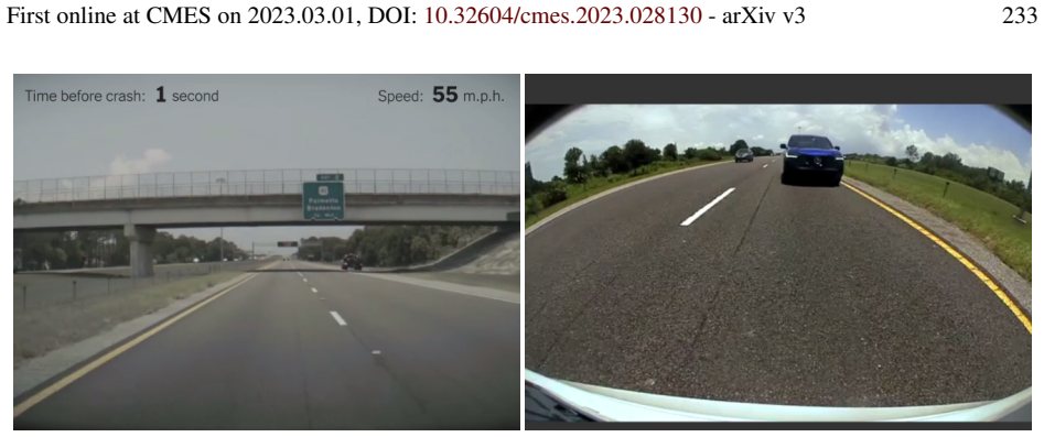
Figure 144. Figure 144: Tesla crash (Section 14.1). July 2020. “Less than a second after the Tesla has slowed to roughly 55 m.p.h. [Left], its rear camera shows a car rapidly approaching [Right]” [382]. There were no moving cars on both lanes in front of the Tesla for a long distance ahead (perhaps a quarter of a mile). See also Figures 143, 145, 146. (Data and video provided by QuantivRisk.) “This process is extremely data-int… view at source ↗
Figure 145
Figure 145. Figure 145: Tesla crash (Section 14.1). July 2020. The fast-coming blue car rear-ended the Tesla, indented its own front bumper, with flying broken glass (or clear plastic) cover shards captured by the Tesla rear camera [382]. See also Figures 143, 144, 146. (Data and video provided by QuantivRisk.) mode. It was too late. The smashed bike scraped a 25-foot wake on the pavement. A person lay crumpled in the road” [39… view at source ↗
Figure 146
Figure 146. Figure 146: Tesla crash (Section 14.1). After hitting the Tesla, the blue car “spun across the highway [Left] and onto the far shoulder [Right],” as another car was coming toward on the right lane (left in photo), but still at a safe distance so not to hit it. [382]. See also Figures 143, 144, 145. (Data and video provided by QuantivRisk.) Similar problems exist with building autonomous boats to ply the oceans witho… view at source ↗
Figure 147
Figure 147. Figure 147: Mayflower autonomous ship (Section 14.1) sailing from Plymouth, UK, planning to arrive at Plymouth, MA, U.S., like the original Mayflower 400 years ago, but instead arriving at Halifax, Nova Scotia, Canada, on 2022 Jun 05, due to mechanical problems [394]. (CC BY￾SA 4.0, Wikipedia, version 16:43, 17 July 2022.) 14.2 Lack of understanding on why deep learning worked Such lack of understanding is described… view at source ↗
Figure 148
Figure 148. Figure 148: Network with infinite width (left) and Gaussian distribution (Right) (Section 6.1, 14.2). “A number of recent results have shown that DNNs that are allowed to become in￾finitely wide converge to another, simpler, class of models called Gaussian processes. In this limit, complicated phenomena (like Bayesian inference or gradient descent dynamics of a con￾volutional neural network) boil down to simple line… view at source ↗
Figure 149
Figure 149. Figure 149: Deepfake images (Section 14.4.1). AI-generated portraits using Generative Ad￾versarial Network (GAN) models. See also [397] [398], Chap. 8, “GAN Fingerprints in Face Image Synthesis.” (Images from ‘This Person Does Not Exist’ site.) 14.4.1 Deepfakes AI software available online helping to create videos that show someone said or did things that the person did not say or do represent a clear danger to demo… view at source ↗
Figure 150
Figure 150. Figure 150: DeepFake detection (Section 14.4.1). Violin plots. • Individual vs machine. The leading model had an accuracy of 65% on 4,000 videos (Col. 1). In Experiment 1 (E1), 5,524 participants were asked to identify a deepfake from each of 56 pairs of videos. The participants had a mean accuracy of 80% (white dot in Col. 2), with 82% of the participants having an accuracy better than that of the leading model (65… view at source ↗
Figure 151
Figure 151. Figure 151: Lack of transparency and irreproducibility (Section 14.7). The table shows many missing pieces of information for the three networks—Lesion, Breast, and Case models—used to detect breast cancer. Learning rate, Section 6.2. Learning-rate schedule, Section 6.3.1, [PITH_FULL_IMAGE:figures/full_fig_p242_151.png] view at source ↗
Figure 152
Figure 152. Figure 152: below [PITH_FULL_IMAGE:figures/full_fig_p268_152.png] view at source ↗
Figure 10
Figure 10. Figure 10: in the online book [PITH_FULL_IMAGE:figures/full_fig_p268_10.png] view at source ↗
Figure 153
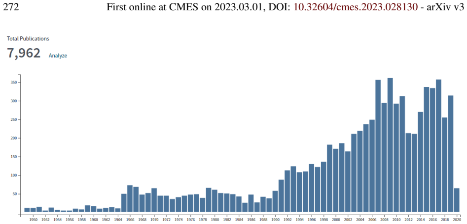
Figure 153. Figure 153: The first two waves of AI, according to [78], p.13, showing the “cybernetics” wave (blue line) started in the 1940s peaked before 1970, then gradually declined toward 2006 and beyond. The results were based on a search for frequency of words in Google Books. It was mentioned, incorrectly, that the work of Rosenblatt (1957-1962) [1]-[2] was limited to one neuron; see [PITH_FULL_IMAGE:figures/full_fig_p27… view at source ↗
Figure 154
Figure 154. Figure 154: Cybernetics papers, (Appendix 4). Web of Science search on 2020.04.15, having more than 100 Web of Science categories. The first paper was [426]. There was no clear wave that crested before 1970, but actually the number of papers in Cybernetics continue to increase over the years. The first paper in 1949 [426] was categorized as Mathematics. More recent papers include Biological Science, e.g., [427], Bui… view at source ↗
Figure 155
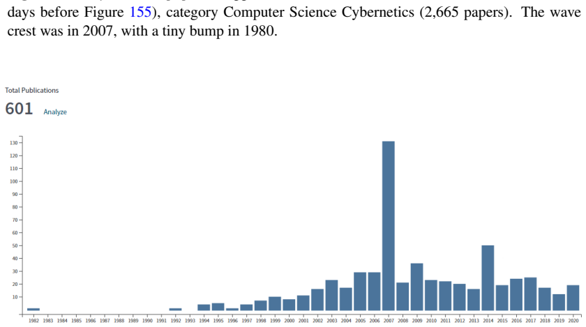
Figure 155. Figure 155: Cybernetics papers, (Appendix 4). Web of Science search on 2020.04.17, ALL Computer-Science categories (3,555 papers): Cybernetics (2,666), Artificial Intelligence (602), Information Systems (432), Theory Methods (300), Interdisciplinary Applications (293), Soft￾ware Engineering (163). The wave crest was in 2007, with a tiny bump in 1980. “... (feedback) control and communication theory pertinent to the … view at source ↗
Figure 156
Figure 156. Figure 156: Cybernetics papers, (Appendix 4). Web of Science search on 2020.04.15 (two days before [PITH_FULL_IMAGE:figures/full_fig_p274_156.png] view at source ↗
Figure 157
Figure 157. Figure 157: Cybernetics papers, (Appendix 4). Web of Science search on 2020.04.15 (two days before [PITH_FULL_IMAGE:figures/full_fig_p274_157.png] view at source ↗
Figure 158
Figure 158. Figure 158: Artificial Intelligence (AI), Machine Learning (ML), and Deep Learning (DL). Cybernetics is broad and encompasses many fields, including AI. See also [PITH_FULL_IMAGE:figures/full_fig_p275_158.png] view at source ↗
read the original abstract

Three recent breakthroughs due to AI in arts and science serve as motivation: An award winning digital image, protein folding, fast matrix multiplication. Many recent developments in artificial neural networks, particularly deep learning (DL), applied and relevant to computational mechanics (solid, fluids, finite-element technology) are reviewed in detail. Both hybrid and pure machine learning (ML) methods are discussed. Hybrid methods combine traditional PDE discretizations with ML methods either (1) to help model complex nonlinear constitutive relations, (2) to nonlinearly reduce the model order for efficient simulation (turbulence), or (3) to accelerate the simulation by predicting certain components in the traditional integration methods. Here, methods (1) and (2) relied on Long-Short-Term Memory (LSTM) architecture, with method (3) relying on convolutional neural networks. Pure ML methods to solve (nonlinear) PDEs are represented by Physics-Informed Neural network (PINN) methods, which could be combined with attention mechanism to address discontinuous solutions. Both LSTM and attention architectures, together with modern and generalized classic optimizers to include stochasticity for DL networks, are extensively reviewed. Kernel machines, including Gaussian processes, are provided to sufficient depth for more advanced works such as shallow networks with infinite width. Not only addressing experts, readers are assumed familiar with computational mechanics, but not with DL, whose concepts and applications are built up from the basics, aiming at bringing first-time learners quickly to the forefront of research. History and limitations of AI are recounted and discussed, with particular attention at pointing out misstatements or misconceptions of the classics, even in well-known references. Positioning and pointing control of a large-deformable beam is given as an example.

Editorial analysis

A structured set of objections, weighed in public.

Desk editor's note, referee report, simulated authors' rebuttal, and a circularity audit. Tearing a paper down is the easy half of reading it; the pith above is the substance, this is the friction.

Referee Report

2 major / 2 minor

Summary. The manuscript is a review paper surveying recent deep learning applications to computational mechanics. It covers hybrid methods that combine traditional PDE discretizations with LSTM (for constitutive modeling and model-order reduction) and CNN (for simulation acceleration), pure ML approaches such as PINNs with attention mechanisms for discontinuous solutions, reviews of LSTM/attention architectures, modern optimizers, and kernel machines (including Gaussian processes and infinite-width networks), plus discussion of AI history, limitations, and misconceptions. An example application to positioning/pointing control of a large-deformable beam is included. The target audience is computational-mechanics experts new to DL, with concepts built from the basics.

Significance. If the literature selection is representative and the coverage balanced, the review would provide a useful on-ramp for mechanics researchers entering DL, explicitly contrasting hybrid and pure-ML strategies and correcting common misconceptions about the classics. The inclusion of both modern architectures and kernel-machine background for advanced readers adds pedagogical value.

major comments (2)
  1. [Abstract] Abstract and opening sections: the central claim that the paper reviews 'many recent developments ... in detail' and supplies the 'state of the art' rests on the assumption of unbiased, comprehensive paper selection up to the 2022 cutoff. No explicit selection methodology, inclusion/exclusion criteria, or discussion of potential gaps (e.g., key LSTM turbulence papers or additional PINN variants) is provided, making it impossible to verify representativeness.
  2. [Introduction (implied by abstract)] The positioning statement that the review brings 'first-time learners quickly to the forefront of research' is load-bearing for the intended contribution, yet the manuscript does not compare its scope or depth against existing surveys in the same area, leaving the incremental value of this particular synthesis unclear.
minor comments (2)
  1. [Abstract] The three motivating AI breakthroughs cited in the abstract are not enumerated explicitly; listing them would strengthen the opening motivation.
  2. Ensure that every cited work is dated no later than the stated 2022 cutoff and that references to the 'classics' are accompanied by the specific misstatements being corrected.

Simulated Author's Rebuttal

2 responses · 0 unresolved

We thank the referee for the constructive comments. We address each major comment below, agreeing that additional clarifications on scope and comparisons to prior surveys will strengthen the manuscript.

read point-by-point responses
  1. Referee: [Abstract] Abstract and opening sections: the central claim that the paper reviews 'many recent developments ... in detail' and supplies the 'state of the art' rests on the assumption of unbiased, comprehensive paper selection up to the 2022 cutoff. No explicit selection methodology, inclusion/exclusion criteria, or discussion of potential gaps (e.g., key LSTM turbulence papers or additional PINN variants) is provided, making it impossible to verify representativeness.

    Authors: We agree that an explicit discussion of literature selection would improve transparency. Although the review was compiled based on relevance to computational mechanics applications up to the 2022 cutoff, we will add a new paragraph in the Introduction describing the general search approach, inclusion focus on solid/fluid mechanics and finite-element contexts, and explicit acknowledgment of potential gaps (e.g., certain turbulence LSTM works or post-cutoff PINN variants). revision: yes

  2. Referee: [Introduction (implied by abstract)] The positioning statement that the review brings 'first-time learners quickly to the forefront of research' is load-bearing for the intended contribution, yet the manuscript does not compare its scope or depth against existing surveys in the same area, leaving the incremental value of this particular synthesis unclear.

    Authors: The manuscript's distinctive elements include the joint treatment of hybrid LSTM/CNN methods with pure PINN approaches, coverage of kernel machines and infinite-width networks, and discussion of AI history with corrections to common misconceptions. We nevertheless recognize the benefit of explicit positioning. We will revise the Introduction to include a concise comparison with related surveys (e.g., those focused primarily on PINNs or data-driven constitutive modeling) and to articulate the incremental synthesis provided here. revision: yes

Circularity Check

0 steps flagged

No circularity: review draws from external citations without internal derivations

full rationale

This is a literature review paper with no original mathematical derivations, predictions, or fitted models presented as results. The central content consists of summaries of external cited works on DL methods for mechanics (LSTM, PINN, etc.), built from basics for the reader. No steps match the enumerated circularity patterns, as there are no equations reducing to inputs by construction, no fitted parameters renamed as predictions, and no load-bearing self-citations that justify a uniqueness theorem or ansatz. The paper is self-contained as a survey against external benchmarks.

Axiom & Free-Parameter Ledger

0 free parameters · 0 axioms · 0 invented entities

As a review article the central content rests on the accuracy and completeness of the surveyed literature rather than new mathematical derivations or postulates.

pith-pipeline@v0.9.0 · 5848 in / 995 out tokens · 26768 ms · 2026-05-24T10:19:58.457659+00:00 · methodology

discussion (0)

Sign in with ORCID, Apple, or X to comment. Anyone can read and Pith papers without signing in.

Forward citations

Cited by 1 Pith paper

Reviewed papers in the Pith corpus that reference this work. Sorted by Pith novelty score.

  1. SLIDE: A machine-learning based method for forced dynamic response estimation of multibody systems

    cs.LG 2024-09 unverdicted novelty 6.0

    SLIDE is a deep learning estimator that truncates initial effects via complex eigenvalues of linearized equations to predict output sequences of damped multibody systems, reporting speedups up to several million times.

Reference graph

Works this paper leans on

286 extracted references · 286 canonical work pages · cited by 1 Pith paper · 38 internal anchors

  1. [2]

    Rosenblatt, F. (1962). Principles of neurodynamics: Perceptrons and the theory of brain mechanisms. Spartan Books. 2, 11, 46, 55, 210, 212, 213, 214, 215, 271

  2. [3]

    Polyak, B. (1964). Some methods of speeding up the convergence of iteration methods . USSR Com- putational Mathematics and Mathematical Physics, 4(5), 1–17. DOI 10.1016/0041-5553(64)90137-5. 2, 10, 11, 85, 89, 90, 91

  3. [4]

    Roose, K. (2022). An A.I.-Generated Picture Won an Art Prize. Artists Aren’t Happy.New York Times, (Sep 2). Original website. 6, 7

  4. [5]

    Jumper, J., Evans, R., Pritzel, A., Green, T., Figurnov, M., et al. (2021). Highly accurate protein structure prediction with AlphaFold. Nature, 596(7873), 583–589. 7

  5. [6]

    J., Guez, A., Sifre, L., et al

    Silver, D., Huang, A., Maddison, C. J., Guez, A., Sifre, L., et al. (2016). Mastering the game of Go with deep neural networks and tree search. Nature, 529(7587), 484+. Original website. 7, 12, 13

  6. [7]

    How Google’s AlphaGo Beat a Go World Champion

    Moyer, C. How Google’s AlphaGo Beat a Go World Champion. 2016 Mar 28, Original website. 7

  7. [8]

    Edwards, B. (2022). DeepMind breaks 50-year math record using AI; new record falls a week later. Ars Technica, (Oct 13). Original website, Internet archive. 7

  8. [9]

    Vu-Quoc, L., Humer, A. (2022). Deep learning applied to computational mechanics: A comprehensive review, state of the art, and the classics. arXiv:2212.08989. 8

  9. [10]

    Roose, K. (2023). Bing (Yes, Bing) Just Made Search Interesting Again. New York Times, (Feb 8). Original website. 8

  10. [11]

    Knight, W. (2023). Meet Bard, Google’s Answer to ChatGPT. WIRED, (Feb 6). Original website. 8

  11. [12]

    Schmidhuber, J. (2015). Deep learning in neural networks: An overview. Neural Networks, 61, 87–

  12. [13]

    8, 36, 38, 52, 223, 224, 225, 272

  13. [14]

    LeCun, Y ., Bengio, Y ., Hinton, G. (2015). Deep learning.Nature, 521(7553), 436–444. 8, 12, 14, 38, 52, 53, 54, 129, 131

  14. [15]

    Khan, S., Yairi, T. (2018). A review on the application of deep learning in system health management. Mechanical Systems and Signal Processing, 107, 241–265. 8

  15. [16]

    Sanchez-Lengeling, B., Aspuru-Guzik, A. (2018). Inverse molecular design using machine learning: Generative models for matter engineering. Science, 361(6400, SI), 360–365. 8

  16. [17]

    S., Beaulieu-Jones, B

    Ching, T., Himmelstein, D. S., Beaulieu-Jones, B. K., Kalinin, A. A., Do, B. T., et al. (2018). Opportu- nities and obstacles for deep learning in biology and medicine. Journal of the Royal Society Interface, 15(141). 8

  17. [18]

    A., Nyhan, M

    Quinn, J. A., Nyhan, M. M., Navarro, C., Coluccia, D., Bromley, L., et al. (2018). Humanitarian applications of machine learning with remote-sensing data: review and case study in refugee settlement mapping. Philosophical Transactions of the Royal Society A-Mathematical Physical and Engineering Sciences, 376(2128). 8

  18. [19]

    F., Higham, D

    Higham, C. F., Higham, D. J. (2019). Deep learning: An introduction for applied mathematicians. SIAM Review, 61(4), 860–891. 8

  19. [20]

    Dayan, P., Abbott, L. (2001). Theoretical Neuroscience: Computational and Mathematical Modeling of Neural Systems. MIT Press. 8, 9, 11, 30, 31, 38, 39, 40, 41, 43, 212, 215, 216, 217, 219

  20. [21]

    Sze, V ., Chen, Y .-H., Yang, T.-J., Emer, J. S. (2017). Efficient Processing of Deep Neural Networks: A Tutorial and Survey. Proceedings of the IEEE, 105(12), 2295–2329. 8, 17, 32, 38, 209

  21. [22]

    Nielsen, M. (2015). Neural Networks and Deep Learning . Determination Press. Original website. Internet archive. 8, 32, 38, 66, 67, 209, 210, 213

  22. [23]

    Rumelhart, D., Hinton, G., Williams, R. (1986). Learning representations by back-propagating errors. Nature, 323(6088), 533–536. 8, 90, 215, 223, 224, 225, 271

  23. [24]

    Ghaboussi, J., Garrett, J., Wu, X. (1991). Knowledge-based modeling of material behavior with neural networks. Journal of Engineering Mechanics-ASCE, 117(1), 132–153. 8, 9, 26, 32, 173, 209, 272

  24. [26]

    Wang, K., Sun, W. C. (2018). A multiscale multi-permeability poroplasticity model linked by recursive homogenizations and deep learning. Computer Methods in Applied Mechanics and Engineering, 334, 337–380. 8, 9, 11, 22, 24, 25, 26, 27, 28, 172, 173, 174, 175, 176, 177, 178, 179, 180, 181, 182, 183, 184

  25. [27]

    Mohan, A., Gaitonde, D. (2018). A deep learning based approach to reduced order modeling for turbulent flow control using LSTM neural networks. arXiv:1804.09269 [physics.comp-ph]. Apr 24. 8, 9, 11, 28, 29, 30, 184, 185, 186, 187, 188, 189, 190, 191, 192

  26. [28]

    Zaman, M., Zhu, J. (1998). A neural network model for a cohesionless soilIn AttohOkine, NO. Arti- ficial Intelligence and Mathematical Methods in Pavement and Geomechanical Systems. International Workshop on Artificial Intelligence and Mathematical Methods in Pavement and Geomechanical Sys- tems, Miami, FL, Nov 05-06, 1998. 9

  27. [29]

    Su, H., Fan, L., Schlup, J. (1998). Monitoring the process of curing of epoxy/graphite fiber composites with a recurrent neural network as a soft sensor. Engineering Applications of Artificial Intelligence , 11(2), 293–306. 9

  28. [30]

    Li, C., Huang, T. (1999). Automatic structure and parameter training methods for modeling of me- chanical systems by recurrent neural networks. Applied Mathematical Modelling , 23(12), 933–944. 9

  29. [31]

    Waszczyszyn, Z. (2000). Neural networks in structural engineering: Some recent results and prospects for applicationsIn Topping, BHV. Computational Mechanics for the Twenty-First Century. 5th Inter- national Conference on Computational Structures Technology/2nd International Conference on Engi- neering Computational Technology, Leuven, Belgium, Sep 06-08, 2000. 9

  30. [32]

    Vaswani, A., Shazeer, N., Parmar, N., Uszkoreit, J., Jones, L., et al. (2017). Attention Is All You Need. CoRR, abs/1706.03762v5. arXiv:1706.03762v5. See Footnote 337. 9, 11, 135, 138, 139, 140, 141, 142, 143, 248

  31. [33]

    Hahnloser, R., Sarpeshkar, R., Mahowald, M., Douglas, R., Seung, S. (2000). Digital selection and analogue amplification coexist in a cortex-inspired silicon circuit (vol 405, pg 947, 2000). Nature, 408(6815), 1012–U24. 9, 39, 219, 221, 222

  32. [34]

    Jarrett, K., Kavukcuoglu, K., Ranzato, M., LeCun, Y . (2009). What is the Best Multi-Stage Architec- ture for Object Recognition?In 2009 IEEE 12th International Conference on Computer Vision (ICCV). IEEE International Conference on Computer Vision. IEEE; IEEE Comp Soc. 12th IEEE International Conference on Computer Vision, Kyoto, JAPAN, SEP 29-OCT 02, 2009. 9, 39

  33. [35]

    Nair, V ., Hinton, G. (2010). Rectified linear units improve restricted boltzmann machines.Proceedings of the 27th International Conference on Machine Learning, Haifa, Israel. 9, 39

  34. [36]

    Little, W. (1974). The existence of persistent states in the brain. Mathematical Biosciences, 19, 101–

  35. [37]

    In Cabrera, B and Gutfreund, H and Kresin, V (eds), From High-Temperature Superconductivity to Microminiature Refrigeration, William Little Symposium on From High-Temperature Supercon- ductivity to Microminiature Refrigeration, Stanford Univ, Stanford, CA, Sep 30, 1995.336. 9, 220

  36. [38]

    Ramachandran, P., Barret, Z., Le, Q. (2017). Searching for Activation Functions. CoRR (Computing Research Repository), abs/1710.05941v2. arXiv:1710.05941v2. See Footnote 337. 9, 52, 219, 221, 222, 223

  37. [40]

    Oishi, A., Yagawa, G. (2017). Computational mechanics enhanced by deep learning. Computer Meth- ods in Applied Mechanics and Engineering, 327, 327–351. 9, 11, 18, 19, 20, 21, 32, 46, 53, 60, 163, 164, 165, 166, 167, 168, 169, 170, 171, 172, 209

  38. [41]

    Zienkiewicz, O., Taylor, R., Zhu, J. (2013). The Finite Element Method: Its Basis and Fundamentals. Oxford: Butterworth-Heineman. 7th edition. 9, 35, 163, 164

  39. [42]

    Barlow, J. (1976). Optimal stress locations in finite-element models. International Journal for Numer- ical Methods in Engineering, 10(2), 243–251. 9

  40. [43]

    Barlow, J. (1977). Optimal stress locations in finite-element models - reply. International Journal for Numerical Methods in Engineering, 11(3), 604. 9

  41. [44]

    Theory Guide

    Abaqus 6.14. Theory Guide. Simulia Systems, Dassault Systèmes. Subsection 3.2.4 Solid isoparamet- ric quadrilaterals and hexahedra. (Website, go to Section Reference, Abaqus Theory Guide, Section 3 Elements, Section 3.2 Continuum elements, then Section 3.2.4.). 9

  42. [45]

    Ghaboussi, J., Garrett, J., Wu, X. (1990). Material Modeling with Neural NetworksIn Pande, GN and Middleton, J. Numerical Methods in Engineering : Theory and Applications, Vol 2. 3rd International Conf on Numerical Methods in Engineering : Theory and Applications ( NUMETA 90 ), Univ Coll Swansea, Swansea, Wales, Jan 07-11, 1990. 9

  43. [46]

    Chen, C. (1989). Applying and validating neural network technology for nondestructive evaluation of materialsIn 1989 IEEE International Conference on Systems, Man, and Cybernetics, Vols 1-3: Con- ference Proceedings. 1989 IEEE International Conf on Systems, Man, and Cybernetics : Decision- Making in Large-Scale Systems, Cambridge, MA, Nov 14-17, 1989. 9

  44. [47]

    Sayeh, M., Viswanathan, R., Dhali, S. (1990). Neural networks for assessment of impact and stress relief on composite-materialsIn Genisio, M. Sixth Annual Conference on Materials Technology: Com- posite Technology. 6th Annual Conf on Materials Technology : Composite Technology, Southern Illinois Univ Carbondale, Carbondale, IL, Apr 10-11, 1990. 9

  45. [48]

    Chen, C., Leclair, S. (1991). A probability neural network (pnn) estimator for improved reliability of noisy sensor data. Journal of Reinforced Plastics and Composites, 10(4), 379–390. 9

  46. [49]

    Kim, Y ., Choi, Y ., Widemann, D., Zohdi, T. (2020). A fast and accurate physics-informed neural network reduced order model with shallow masked autoencoderer. ( Sep 28). Version 2, 2020.09.28: arXiv:2009.11990v2, 2009.11990. 9, 10, 11, 193, 194, 195, 196, 197, 198, 199, 200, 201, 203, 205, 206, 207

  47. [50]

    Kim, Y ., Choi, Y ., Widemann, D., Zohdi, T. (2020). Efficient nonlinear manifold reduced order model. (Nov 13). arXiv:2011.07727, 2011.07727. 9, 10, 11, 193

  48. [51]

    Robbins, H., Monro, S. (1951b). Stochastic approximation. Annals of Mathematical Statistics, 22(2),

  49. [52]

    Nesterov, I. (1983). A method of the solution of the convex-programming problem with a speed of convergence O(1/k2). Doklady Akademii Nauk SSSR, 269(3), 543–547. In Russian. 10, 89, 91

  50. [53]

    Nesterov, Y . (2018). Lecture on Convex Optimization. 2nd edition. Switzerland: Springer Nature. 10, 89, 91

  51. [54]

    Duchi, J., Hazan, E., Singer, Y . (2011). Adaptive Subgradient Methods for Online Learning and Stochastic Optimization. Journal of Machine Learning Research, 12, 2121–2159. 10, 105

  52. [55]

    Tieleman, T., Hinton, G. (2012). Lecture 6e, rmsprop: Divide the gradient by a running average of its recent magnitude. Youtube video, time 5:54. Lecture notes, p.29: Original website, Internet archive. 10, 108

  53. [56]

    Zeiler, M. D. (2012). ADADELTA: An adaptive learning rate method. ( Dec 22). arXiv:1212.5701. 10, 106, 108, 109

  54. [58]

    Loshchilov, I., Hutter, F. (2019). Decoupled weight decay regularization. (Jan 4). arXiv:1711.05101v3. OpenReview. 10, 85, 87, 92, 93, 99, 106, 109, 115, 116, 117, 123

  55. [59]

    Bahdanau, D., Cho, K., Bengio, Y . (2015). Neural machine translation by jointly learning to align and translate. CoRR, abs/1409.0473. arXiv:1409.0473. 11, 135, 136, 137, 138

  56. [60]

    Furshpan, E., Potter, D. (1957). Mechanism of nerve-impulse transmission at a crayfish synapse. Nature, 180(4581), 342–343. 11, 222

  57. [61]

    Furshpan, E., Potter, D. (1959b). Slow post-synaptic potentials recorded from the giant motor fibre of the crayfish. Journal of Physiology-London, 145(2), 326–335. 11, 222

  58. [62]

    Gershgorn, D. (2017). The data that transformed AI research—and possibly the world. Quartz, (Jul 26). Original website. Internet archive (blurry images). 11, 13

  59. [63]

    He, K., Zhang, X., Ren, S., Sun, J. (2015). Delving Deep into Rectifiers: Surpassing Human-Level Performance on ImageNet Classification. CoRR, abs/1502.01852. arXiv:1502.01852, 1502.01852. 12, 40, 70, 206, 220

  60. [64]

    Russakovsky, O., Deng, J., Su, H., Krause, J., Satheesh, S., et al. (2015). ImageNet Large Scale Visual Recognition Challenge. International Journal of Computer Vision, 115(3), 211–252. 12, 13

  61. [65]

    Park, E., Liu, W., Russakovsky, O., Deng, J., Li, F., et al. (2017). ImageNet Large scale visual recogni- tion challenge (ILSVRC) 2017, Overview. ILSVRC 2017, (Jul 26). Original website Internet archive. 12, 13

  62. [66]

    Science’s 2021 Breakthrough: AI-powered Protein Prediction

    Beckwith, W. Science’s 2021 Breakthrough: AI-powered Protein Prediction. 2022 Dec 17, Original website. 11, 12

  63. [67]

    DeepMind, 2022 Jul 28, Original website, Internet archive

    AlphaFold reveals the structure of the protein universe. DeepMind, 2022 Jul 28, Original website, Internet archive. 12

  64. [68]

    DeepMind’s AI predicts structures for a vast trove of proteins

    Callaway, E. DeepMind’s AI predicts structures for a vast trove of proteins. 2021 Jul 21, Original website. 12

  65. [69]

    The Guardian view on the future of AI: Great power, great irresponsibility

    Editorial (2019). The Guardian view on the future of AI: Great power, great irresponsibility. The Guardian, (Jan 01). Original website. Internet archive. 12, 236, 237

  66. [70]

    Silver, D., Hubert, T., Schrittwieser, J., Antonoglou, I., Lai, M., et al. (2018). A general reinforcement learning algorithm that masters chess, shogi, and Go through self-play.Science, 362(6419), 1140+. 12

  67. [71]

    A., Veness, J., et al

    Mnih, V ., Kavukcuoglu, K., Silver, D., Rusu, A. A., Veness, J., et al. (2015). Human-level control through deep reinforcement learning. Nature, 518(7540), 529–533. 13

  68. [72]

    P., Buesing, L., Guez, A., et al

    Racaniere, S., Weber, T., Reichert, D. P., Buesing, L., Guez, A., et al. (2017). Imagination-Augmented Agents for Deep Reinforcement Learning. In Guyon, I and Luxburg, UV and Bengio, S and Wallach, H and Fergus, R and Vishwanathan, S and Garnett, R, editor,Advances in Neural Information Processing Systems 30 (NIPS 2017), volume 30 of Advances in Neural In...

  69. [73]

    Silver, D., Schrittwieser, J., Simonyan, K., Antonoglou, I., Huang, A., et al. (2017). Mastering the game of Go without human knowledge. Nature, 550(7676), 354+. 13

  70. [74]

    Artificial intelligence - hype, hope and fear

    Cellan-Jones, Rory (2017). Artificial intelligence - hype, hope and fear. BBC, (Oct 16). Original website. Internet archive. 13

  71. [75]

    Campbell, M. (2018). Mastering board games. A single algorithm can learn to play three hard board games. Science, 362(6419), 1118. 13

  72. [76]

    Why artificial intelligence is enjoying a renaissance

    The Economist (2016). Why artificial intelligence is enjoying a renaissance. ( Jul 15 ). (https://goo.gl/Grkofq). 13, 54, 226

  73. [77]

    From not working to neural networking

    The Economist (2016). From not working to neural networking. ( Jun 25). (https://goo.gl/z1c9pc). 13, 52, 54, 226

  74. [79]

    Hardesty, L. (2017). Explained: Neural networks. MIT News, (Apr 14). Original website. Internet archive. 13, 210

  75. [80]

    Goodfellow, I., Bengio, Y ., Courville, A. (2016). Deep Learning. Cambridge, MA: The MIT Press. 14, 16, 17, 27, 32, 34, 35, 36, 37, 38, 39, 40, 44, 46, 47, 48, 49, 52, 53, 54, 55, 56, 57, 58, 59, 60, 61, 62, 65, 67, 69, 70, 72, 73, 75, 76, 77, 78, 84, 85, 86, 87, 89, 90, 91, 92, 93, 99, 100, 102, 104, 106, 108, 109, 112, 114, 115, 126, 127, 128, 129, 131,...

  76. [81]

    Ford, K. (2018). Architects of Intelligence: The truth about AI from the people building it . Packt Publishing. 14, 16, 221, 223, 224, 225, 235

  77. [82]

    E., Nocedal, J

    Bottou, L., Curtis, F. E., Nocedal, J. (2018). Optimization Methods for Large-Scale Machine Learning. SIAM Review, 60(2), 223–311. 14, 76, 78, 84, 85, 87, 93, 106, 108, 109

  78. [83]

    Khullar, D. (2019). A.I. Could Worsen Health Disparities. New York Times, (Jan 31). Original website. 14

  79. [84]

    Kornfield, M., Firozi, P. (2020). Artificial intelligence use is growing in the U.S. healthcare system. Washington Post, (Feb 24). Original website. 14

  80. [85]

    Lee, K. (2018a). AI Superpowers: China, Silicon Valley, and the New World Order. Houghton Mifflin Harcourt. 14

Showing first 80 references.