Scaling Laws of Quantum Information Lifetime in Monitored Quantum Dynamics
Pith reviewed 2026-05-19 07:48 UTC · model grok-4.3
The pith
Continuous monitoring of the environment lets quantum information lifetime grow exponentially with system size, independent of bath size.
A machine-rendered reading of the paper's core claim, the machinery that carries it, and where it could break.
Core claim
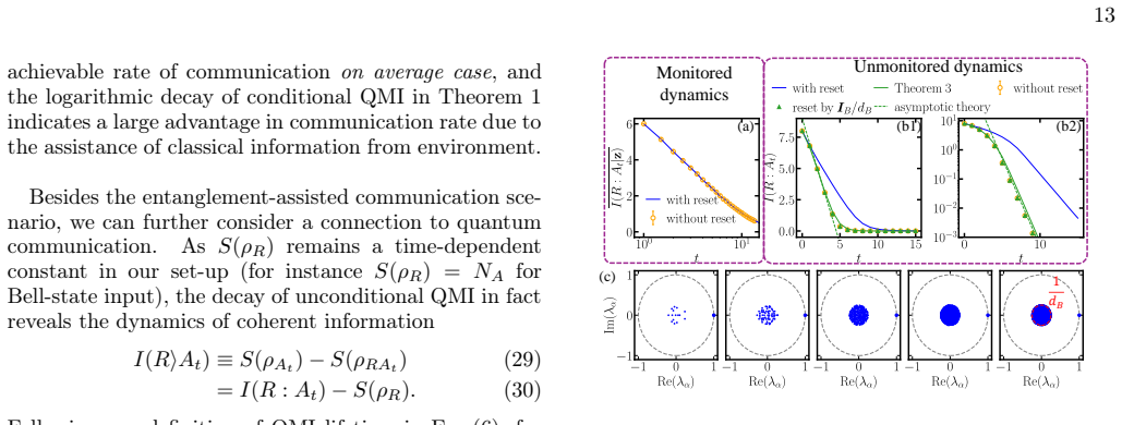
Starting from a maximally entangled state, the lifetime of quantum mutual information between system and reference scales exponentially with system size under continuous bath monitoring via mid-circuit measurements, for typical Haar random unitaries; without monitoring the lifetime grows at most linearly with system size and inversely with bath size.
What carries the argument
The scaling of quantum mutual information lifetime under continuous mid-circuit monitoring of the bath, proven analytically for Haar-random unitaries and checked in random circuits and chaotic Hamiltonians.
If this is right
- Quantum diffusion models and reservoir computing can retain input information for times that grow with system size rather than saturating.
- Quantum communication protocols gain a route to protect entanglement even when the environment is large.
- Monitored circuits in the weak-measurement limit inherit the same exponential lifetime scaling.
- Hardware experiments on IBM devices already confirm a measurable gap between monitored and unmonitored information persistence.
Where Pith is reading between the lines
- Monitoring strategies could be combined with existing error-correction codes to extend coherence times without increasing code size.
- The two-scale transition may appear in other monitored many-body systems beyond circuits, offering a diagnostic for measurement strength.
- Larger-scale simulations or future hardware could test whether the exponential scaling survives when the unitaries are only approximately random.
Load-bearing premise
The analytic proof requires the dynamics to be typical of Haar-random unitaries, which assumes sufficient randomness that may not hold for every possible Hamiltonian.
What would settle it
A direct numerical or experimental measurement showing that monitored lifetime remains linear or sub-linear with system size in a chaotic Hamiltonian system would contradict the central scaling claim.
Figures


read the original abstract
Quantum information is typically fragile under measurements and environmental coupling. Remarkably, we find that its lifetime can scale exponentially with system size when the environment is continuously monitored via mid-circuit measurements -- regardless of bath size. Starting from a maximally entangled state with a reference, we analytically prove this exponential scaling for typical Haar random unitaries and confirm it through numerical simulations in both random unitary circuits and chaotic Hamiltonian systems. In the absence of bath monitoring, the lifetime exhibits a markedly different scaling: it grows at most linearly -- or remains constant -- with system size and decays inversely with the bath size. We further extend our findings numerically to a broad class of initial states. In the intermediate regime of partial monitoring, we identify and prove a two-scale transition, where the QMI decays logarithmically at microscopic time scales but linearly at macroscopic time scales.} We discuss implications for {monitored quantum circuits in the weak measurement limit, quantum algorithms such as quantum diffusion models and quantum reservoir computing, and quantum communication. Finally, we experimentally verify the gap of persisted information on IBM Quantum hardwares.
Editorial analysis
A structured set of objections, weighed in public.
Referee Report
Summary. The manuscript claims that continuous mid-circuit monitoring of the environment in quantum dynamics protects quantum information, yielding a lifetime (via quantum mutual information with a reference) that scales exponentially with system size independent of bath size. This is analytically proven for typical Haar-random unitaries starting from maximally entangled states, numerically confirmed in random unitary circuits and chaotic Hamiltonians, extended to other initial states, and shown to exhibit a two-scale (logarithmic then linear) transition under partial monitoring. Without monitoring the scaling is at most linear/constant and inversely dependent on bath size; experimental verification on IBM Quantum hardware is also reported.
Significance. If the central claims hold, the work would be significant for monitored quantum dynamics and quantum information science. The analytical proof for Haar-random unitaries supplies a rigorous, parameter-free foundation, while the numerical checks across circuit and Hamiltonian models plus hardware experiments add reproducibility and falsifiability. The reported independence from bath size and implications for quantum algorithms (diffusion models, reservoir computing) and communication would be noteworthy contributions if the scope beyond maximal scrambling is clarified.
major comments (2)
- [Abstract / Analytical Proof] Abstract and analytical proof section: the headline claim is for monitored quantum dynamics in general, yet the analytic result is restricted to typical Haar-random unitaries (maximal scrambling). The manuscript must supply either an extension argument or explicit caveats showing why the protection mechanism survives for non-random or weakly chaotic Hamiltonians, as the numerical evidence alone cannot establish this.
- [Numerical Simulations] Numerical simulations for chaotic Hamiltonians: system sizes are modest by necessity; the manuscript should include a finite-size scaling collapse or explicit comparison of exponential versus power-law fits (with R² or similar metrics) to demonstrate that the observed growth is not consistent with sub-exponential alternatives.
minor comments (2)
- [Introduction] Define QMI and all acronyms at first use; clarify the precise definition of 'lifetime' (e.g., time to reach a fixed QMI threshold) in the main text.
- [Experimental Verification] Experimental section: specify the IBM Quantum device names, circuit depths, number of shots, and any error-mitigation protocol used to support the hardware verification claim.
Simulated Author's Rebuttal
We thank the referee for the careful reading and constructive suggestions. We address each major comment below and will revise the manuscript to improve clarity on the scope of the analytic results and to strengthen the numerical evidence.
read point-by-point responses
-
Referee: [Abstract / Analytical Proof] Abstract and analytical proof section: the headline claim is for monitored quantum dynamics in general, yet the analytic result is restricted to typical Haar-random unitaries (maximal scrambling). The manuscript must supply either an extension argument or explicit caveats showing why the protection mechanism survives for non-random or weakly chaotic Hamiltonians, as the numerical evidence alone cannot establish this.
Authors: We agree that the rigorous analytic proof applies specifically to typical Haar-random unitaries. In the revision we will add explicit caveats in the abstract, introduction, and discussion sections clarifying this scope. We will also include a short argument that the protection arises from the scrambling properties shared by both the Haar ensemble and sufficiently chaotic Hamiltonians, as evidenced by the consistent numerical behavior across models; a complete analytic extension to arbitrary Hamiltonians is beyond the present scope but will be noted as an open direction. revision: yes
-
Referee: [Numerical Simulations] Numerical simulations for chaotic Hamiltonians: system sizes are modest by necessity; the manuscript should include a finite-size scaling collapse or explicit comparison of exponential versus power-law fits (with R² or similar metrics) to demonstrate that the observed growth is not consistent with sub-exponential alternatives.
Authors: We acknowledge the limitation imposed by modest system sizes in the Hamiltonian simulations. In the revised manuscript we will add explicit comparisons of exponential versus power-law fits to the quantum mutual information lifetime data, including R² or equivalent goodness-of-fit metrics. Where computationally feasible we will also present a finite-size scaling analysis to further support the exponential scaling over sub-exponential alternatives. revision: yes
Circularity Check
No circularity: analytical proof for Haar-random unitaries stands independently of numerics and uses standard averaging.
full rationale
The derivation begins from a maximally entangled reference-system state and applies standard Haar averaging over the unitary group to prove exponential lifetime scaling under continuous bath monitoring. This averaging step is a conventional technique in quantum information and does not presuppose the target scaling law or reduce to a fitted parameter. Numerical simulations on random circuits and chaotic Hamiltonians are presented as separate confirmation rather than inputs to the analytic result. The contrast with the unmonitored case (linear or constant scaling) follows directly from the absence of the monitoring protocol in the same averaging framework. No self-citation chains, ansatz smuggling, or uniqueness theorems imported from prior author work are invoked as load-bearing steps for the central claim. The result is therefore self-contained against external benchmarks.
Axiom & Free-Parameter Ledger
Lean theorems connected to this paper
-
IndisputableMonolith/Foundation/RealityFromDistinction.leanreality_from_one_distinction unclear?
unclearRelation between the paper passage and the cited Recognition theorem.
Theorem 1 ... EHaar I(R : At|z) ≳ 2NA − 2 log2 [(1 − 1/dB)t + 1] ... τcond ≳ Ω(exp(NA))
-
IndisputableMonolith/Cost/FunctionalEquation.leanwashburn_uniqueness_aczel unclear?
unclearRelation between the paper passage and the cited Recognition theorem.
Theorem 2 ... EHaar I2(R : At) ≃ 2NA − t NB (early time)
What do these tags mean?
- matches
- The paper's claim is directly supported by a theorem in the formal canon.
- supports
- The theorem supports part of the paper's argument, but the paper may add assumptions or extra steps.
- extends
- The paper goes beyond the formal theorem; the theorem is a base layer rather than the whole result.
- uses
- The paper appears to rely on the theorem as machinery.
- contradicts
- The paper's claim conflicts with a theorem or certificate in the canon.
- unclear
- Pith found a possible connection, but the passage is too broad, indirect, or ambiguous to say the theorem truly supports the claim.
Forward citations
Cited by 1 Pith paper
-
Anticoncentrated $n$-bit distribution from $\log(n)$ qubits
n-bit anticoncentrated distributions can be generated from O(log n) qubits via a holographic protocol of interleaved random unitaries and mid-circuit measurements.
Reference graph
Works this paper leans on
-
[1]
W. W. Ho and S. Choi, Phys. Rev. Lett.128, 060601 (2022)
work page 2022
-
[2]
J. S. Cotler, D. K. Mark, H.-Y. Huang, F. Hernandez, J. Choi, A. L. Shaw, M. Endres, and S. Choi, PRX quan- tum 4, 010311 (2023)
work page 2023
-
[3]
Y. Li, X. Chen, and M. P. Fisher, Phys. Rev. B100, 134306 (2019)
work page 2019
- [4]
-
[5]
A. R. Calderbank and P. W. Shor, Phys. Rev. A54, 1098 (1996)
work page 1996
-
[6]
Google Quantum AI and Collaborators, Nature638, 920 (2025)
work page 2025
- [7]
-
[8]
A. D. Córcoles, M. Takita, K. Inoue, S. Lekuch, Z. K. Minev, J. M. Chow, and J. M. Gambetta, Phys. Rev. Lett. 127, 100501 (2021)
work page 2021
-
[9]
M. DeCross, E. Chertkov, M. Kohagen, and M. Foss-Feig, Phys. Rev. X13, 041057 (2023)
work page 2023
- [10]
- [11]
-
[12]
H. Buhrman, M. Folkertsma, B. Loff, and N. M. Neu- mann, Quantum8, 1552 (2024)
work page 2024
-
[13]
K. C. Smith, A. Khan, B. K. Clark, S. Girvin, and T.-C. Wei, PRX Quantum5, 030344 (2024)
work page 2024
- [14]
- [15]
-
[16]
J. Chen, H. I. Nurdin, and N. Yamamoto, Physical Re- view Applied14, 024065 (2020)
work page 2020
-
[17]
F. Hu, S. A. Khan, N. T. Bronn, G. Angelatos, G. E. Rowlands, G. J. Ribeill, and H. E. Türeci, Nat. Commun. 15, 7491 (2024)
work page 2024
-
[18]
C. H. Bennett, P. W. Shor, J. A. Smolin, and A. V. Thap- liyal, IEEE Trans. Inf. Theo.48, 2637 (2002)
work page 2002
-
[19]
K. Nakajima, K. Fujii, M. Negoro, K. Mitarai, and M. Kitagawa, Phys. Rev. Applied11, 034021 (2019)
work page 2019
- [20]
- [21]
-
[22]
T. Yasuda, Y. Suzuki, T. Kubota, K. Nakajima, Q. Gao, W. Zhang, S. Shimono, H. I. Nurdin, and N. Yamamoto, arXiv:2310.06706 [quant-ph] (2023)
-
[23]
R. Martínez-Peña and J.-P. Ortega, Physical Review E 107, 035306 (2023)
work page 2023
-
[24]
Jaeger, GMD-German National Research Institute for Computer Science (2002) (2002)
H. Jaeger, GMD-German National Research Institute for Computer Science (2002) (2002)
work page 2002
-
[25]
S. Ganguli, D. Huh, and H. Sompolinsky, Proceedings of the National Academy of Sciences105, 18970–18975 (2008)
work page 2008
- [26]
-
[27]
D. Verstraeten, J. Dambre, X. Dutoit, and B. Schrauwen, in The 2010 International Joint Conference on Neural Networks (IJCNN)(IEEE, 2010) p. 1–8
work page 2010
-
[28]
M. Inubushi and K. Yoshimura, Scientific Reports 7, 10.1038/s41598-017-10257-6 (2017)
-
[29]
E. P. Wigner, inPhilosophical reflections and syntheses (Springer, 1995) pp. 247–260
work page 1995
- [30]
-
[31]
[17], these are referred to as the Memory (M) and Readout (R) subsystems
In the context of the NISQRC algorithm of Ref. [17], these are referred to as the Memory (M) and Readout (R) subsystems
- [32]
- [33]
-
[34]
Nature622, 481 (2023)
work page 2023
-
[35]
R. Kukulski, I. Nechita, Ł. Pawela, Z. Puchała, and K. Życzkowski, J. Math. Phys.62 (2021)
work page 2021
- [36]
-
[37]
Unitary designs from statistical mechanics in random quantum circuits
N. Hunter-Jones, arXiv:1905.12053 (2019)
work page internal anchor Pith review Pith/arXiv arXiv 1905
-
[38]
M. M. Wilde,Quantum information theory(Cambridge university press, 2013)
work page 2013
- [39]
-
[40]
R.Belyansky, P.Bienias, Y.A.Kharkov, A.V.Gorshkov, and B. Swingle, Phys. Rev. Lett.125, 130601 (2020)
work page 2020
-
[41]
A. Javadi-Abhari, M. Treinish, K. Krsulich, C. J. Wood, J. Lishman, J. Gacon, S. Martiel, P. D. Na- tion, L. S. Bishop, A. W. Cross, B. R. Johnson, and J.M.Gambetta,QuantumcomputingwithQiskit(2024), arXiv:2405.08810 [quant-ph]
work page internal anchor Pith review Pith/arXiv arXiv 2024
- [42]
-
[43]
Y. Li, Y. Zou, P. Glorioso, E. Altman, and M. P. Fisher, Phys. Rev. Lett.130, 220404 (2023)
work page 2023
- [44]
- [45]
-
[46]
S.-X. Zhang, J. Allcock, Z.-Q. Wan, S. Liu, J. Sun, H. Yu, X.-H. Yang, J. Qiu, Z. Ye, Y.-Q. Chen,et al., Quantum 7, 912 (2023). Appendix A: Equivalence of with/without reset in measurement-conditioned QMI In this section, we prove that the dynamics of measurement-conditioned QMI remains the same regard- less of reset or not. Similar to Eq. (1), the condit...
work page 2023
-
[47]
dA(1 + dB) 1 + d2 AdB + 1 − d2 A dA(1 + d2 AdB) dB(d2 A − 1) d2 Ad2 B − 1 t# + log2
Pure-state reset strategy For pure-state reset strategy, without loosing generality, we simply assume in every step, the bath system is reset to the trivial product state|0⟩. From the equivalence relation in Fig. 15, we can write out the linear mapE as E = X a,b t−1Y k=0 ⟨ak+1bk+1|Uk|ak0⟩ |at⟩At ⊗t−1 k=0 |bk+1⟩Bk+1 ⟨a0|A0 , (E2) where a = (a0, · · · , at)...
-
[48]
dB − 1 dA d2 A − 1 d2 Ad2 B − 1 t + 1 dA # + log2
Fully-mixed state reset strategy In this part, we focus on a different reset strategy, the bath system is initialized with a fully-mixed stateω = IB/dB starting from the second step. Similar to the derivation in pure-state reset strategy, we first write out the linear mapE (shown by blue box in Fig. 17) as E = X a,b t−1Y k=0 ⟨ak+1b2k+1|Uk|akb2k⟩ |at⟩At ⟨a...
discussion (0)
Sign in with ORCID, Apple, or X to comment. Anyone can read and Pith papers without signing in.