REVIEW 4 major objections 4 minor 1 cited by
A hybrid quantum-classical algorithm finds a 49-qubit ground state that standard classical heuristics miss.
Reviewed by Pith at T0; open to challenge. T0 means a machine referee read the full paper against a public rubric. the ladder, T0–T4 →
T0 review · deepseek-v4-flash
2026-08-02 19:06 UTC pith:4C3EEMND
load-bearing objection A real result, honestly scoped in the text, but the abstract overreaches: the quantum hardware is not load-bearing because the same configurations can be sampled from the classically compiled MPS targets. the 4 major comments →
Observation of Improved Accuracy over Classical Sparse Ground-State Solvers using a Quantum Computer
The pith
A machine-rendered reading of the paper's core claim, the machinery that carries it, and where it could break.
Core claim
The central claim is that a sample-based quantum diagonalization algorithm can outperform standard selected configuration interaction heuristics in practice. The paper constructs a class of local Hamiltonians with sparse ground states and designs one instance where perturbation-theory-based SCI solvers get stuck: partial ground states obtained from subspaces are separated from the full ground state by a level crossing, so first-order selection criteria discard the very configurations needed. On a 49-qubit instance, none of the off-the-shelf SCI methods reach the exact energy, while SKQD, run on a 49-qubit processor, does. The authors are careful to note that the problem is still solvable cla
What carries the argument
The mechanism that carries the argument is a Hamiltonian construction with a level-crossing twist. Each patch Hamiltonian has an 8x8 leading block whose lowest eigenvector, restricted to any proper principal submatrix, lives only on the first two configurations; the true ground state appears only when the final off-diagonal coupling connects all eight support configurations, causing a level crossing. This makes the SCI cost function, based on first-order perturbation theory, vanish for the needed configurations even when they are proposed. SKQD bypasses this by sampling from time-evolved states U^k|x0>, whose support covers the true ground-state configurations, and then performing classical
Load-bearing premise
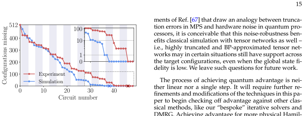
The sampling circuits actually used on the processor are approximate quantum compilations of the time-evolved Krylov states, with fidelities decaying from 0.97 to 0.08; the formal convergence guarantee of SKQD applies to the exact evolution U^k, and the paper validates that the compiled circuits still cover the support only through tensor-network simulation that already knows the 512 support configurations.
What would settle it
Run any of CIPSI, HCI, ASCI, or TrimCI with a hyperparameter setting that reaches the exact ground-state energy using a diagonalization dimension at or below the roughly 10.3 million filtered configurations SKQD used; the claimed superiority over SCI would collapse. A cleaner falsifier would be to replace the approximate compiled circuits in SKQD with random circuits of the same depth and show they still produce the exact energy, which would indicate the success is not due to the Krylov structure.
If this is right
- If SKQD routinely outperforms SCI on sparse ground-state problems, sample-based quantum diagonalization becomes a viable path to classically verifiable quantum advantage for this problem family.
- The paper's Hamiltonian family provides a reusable benchmark class for comparing quantum and classical sparse ground-state solvers on problems with known ground states and known support.
- Because SKQD's energies are variational and the projection matrix is computed classically from sampled configurations, the advantage over SCI is verifiable without trusting the quantum hardware.
- The result shows noise need not destroy the sampling advantage: the quantum experiment succeeded even though the compiled circuits used to approximate the Krylov states have fidelities decaying to 0.08.
- The paper reframes the target for near-term quantum advantage: for sparse ground-state problems, beating standard heuristics is a meaningful milestone, even if the problem remains solvable by DMRG or custom classical solvers.
Where Pith is reading between the lines
- The level-crossing design is a concrete, searchable signature for classically hard sparse ground-state instances: look for Hamiltonians where partial ground states of configuration subspaces differ qualitatively from the full ground state, so perturbation-based expansion stalls.
- The experimental success may depend on the approximate compiled circuits preserving support coverage even at low global fidelity; a natural test is to rerun SKQD with different approximate circuits (or no AQC) to see whether support coverage, not fidelity, is the operative resource.
- The advantage over SCI is synthetic and may not transfer to physical chemistry or condensed-matter Hamiltonians; a testable extension is to apply SKQD to Hamiltonians with long-range support correlations to see whether DMRG also fails, as the paper suggests for future work.
- The paper's custom classical solvers (truncated Arnoldi and diagonal ranking) already beat SKQD in diagonalization dimension, so the next practical question is whether the level-crossing construction can be hardened against these non-perturbative methods as well.
Editorial analysis
A structured set of objections, weighed in public.
Referee Report
Summary. The paper constructs a class of local, heavy-hex-compatible Hamiltonians with sparse product ground states, engineered so that partial subspace ground states are uninformative for SCI-type solvers. On a 49-qubit instance, the authors report that CIPSI, ASCI, HCI, and TrimCI — after hyperparameter sweeps — do not reach the exact ground-state energy, while sample-based Krylov quantum diagonalization (SKQD) executed on an IBM Heron processor reaches it with a Krylov dimension of 17. The paper also describes two custom classical iterative solvers and DMRG that do solve the instance, and it explicitly discloses that direct tensor-network simulation of the sampling circuits can recover all support configurations. The stated claim is scoped to outperforming off-the-shelf SCI heuristics, not to a full quantum advantage.
Significance. If taken at face value, this is the first experimental demonstration that a sample-based Krylov subspace workflow can beat standard SCI heuristics on a nontrivial sparse ground-state instance, with the useful property that the reported energies are variational and classically verifiable. The paper is unusually transparent: it provides the Hamiltonian, detailed hyperparameter sweeps, a full proof of the truncated power method, and an explicit admission that other classical methods (DMRG, custom iterative solvers, tensor-network simulation of the quantum circuits) solve the instance. The significance is therefore not quantum advantage over all classical methods, but a concrete, reproducible benchmark separating SCI-type heuristics from a broader class of methods. That significance is real but substantially weakened by the fact that the configuration basis used by the quantum experiment was already available classically through the AQC/MPS pipeline.
major comments (4)
- [§IV B, App. B 2, App. C] The load-bearing information for the successful diagonalization — the 512 support configurations — is obtained from AQC circuits whose target states are MPS representations computed classically. App. C states explicitly: “Drawing 10^5 samples from |ψ_k^(χ=256)> for each k≤20 reliably yields all support configurations.” The quantum processor samples low-fidelity (F down to 0.08, Table I) versions of these classically known states. Thus the experiment does not establish that the quantum samples are responsible for the improvement over SCI; a classical MPS+AQC sampling pipeline can produce the same configuration basis. The abstract's sentence “a quantum algorithm can outperform classical SCI methods” invites a stronger inference than the experiment supports. This should be addressed by either comparing the quantum result against a classical MPS-sampling baseline with comparable resource acc
- [§II A, Algorithm 1; Table I; §IV B] The rigorous SKQD convergence guarantee from Ref. [30] applies to sampling from the exact Krylov states U^k|x0⟩. The circuits actually executed are AQC-compiled approximations with fidelities as low as 0.08, optionally followed by 0–2 Trotter steps. These circuits are a heuristic variant for which no theorem is offered. The paper validates sufficiency only empirically, using tensor-network simulations that already know the support configurations (App. C, Fig. 7). This matters because if the low-fidelity circuits did not cover the support, the quantum experiment would fail while the classical narrative would remain intact. To make the central claim solid, the authors should either provide a formal statement covering the compiled circuits or clearly state that the experiment demonstrates a heuristic version of SKQD, with the convergence guarantee as motivation rather than as a rigorous cer
- [§IV D, App. D 3–4] The text claims that CIPSI and HCI fail “even for arbitrarily small selection thresholds.” The evidence consists of finite sweeps (ε down to 10^-17 for CIPSI and 10^-20 for HCI) that show saturation of the subspace dimension and energy error. This is not a proof for all positive thresholds, and the literal ε→0 limit reduces to unselected full CI with exponential cost, which is outside the SCI heuristic regime. The claim should be weakened to something like “over the range of thresholds that can be affordably explored” or supplemented with an explicit lower bound on the positive threshold needed to reach the exact energy. As stated, the claim is stronger than the numerical evidence.
- [§IV A, Eq. (22)] The parameters m1, m2, j1 were chosen “based on a sweep to identify regions of classical hardness.” This is an adversarial benchmark design, not a physically motivated instance. This is acceptable for a first demonstration, and the conclusion section acknowledges the limited generality, but the main-text framing (“we construct a class of local Hamiltonian problems” and “SCI fails”) should make clearer that the instance was selected precisely because it is hard for SCI, and that the finding is therefore not evidence about typical or physical Hamiltonians.
minor comments (4)
- [§IV B] “with just 97 shots across the kAQC =1, ..., 16 subset” appears to be a typo; the appendices consistently report 97 million shots. Please correct.
- [§IV B vs App. E] The main text calls the processor “Heron R3,” while App. E says “Heron r2.” Please reconcile.
- [Fig. 5 and elsewhere] Several exponent labels appear as “10°4” etc., presumably intended as 10^{-4}. Please fix the typography.
- [Ref. [30]] The author list contains “W. K. Petar Jurcevic,” which looks like an error; likely the intended author is Petar Jurcevic.
Circularity Check
No circular derivation: the SCI failure is engineered and the SKQD energy is variational; disclosed classical simulability weakens significance but is not circular.
full rationale
The paper's central comparison is a benchmark construction, not a derived prediction. The exact ground state and its 512-configuration support are fixed first (Algorithms 2-3, Eq. (4)), and H is built so that this state is the ground state by construction. That makes the exact answer known, but it does not make the subsequent claim circular: SCI's failure is an observed/calculated consequence of the deliberately chosen H_S0 (Section III A, Eq. (8): the first-order numerator vanishes for i=3..7), and SKQD's success is independently verifiable because the reported energy is obtained by classical projection/diagonalization on the sampled configurations and is variational. The paper is transparent that the Hamiltonian is classically solvable by DMRG, truncated Arnoldi, diagonal ranking, and direct tensor-network simulation of the SKQD circuits; App. C states 'Drawing 10^5 samples from |ψ^{χ=256}_k⟩ for each k≤20 reliably yields all support configurations.' This shows the quantum hardware is not load-bearing for the demonstrated accuracy and limits the significance of 'outperform SCI', but it is a disclosed scope limitation rather than a circular reduction. The SKQD convergence guarantee is cited to the authors' prior work [30], but this self-citation is not load-bearing for the experimental result: the energy comparison rests on the variational projection, not on the theorem. There is no equation here that is equivalent to its own input and no fitted parameter renamed as a prediction.
Axiom & Free-Parameter Ledger
free parameters (5)
- H_S0 matrix entries a, b, c (Eq. 5) =
a=0.90694271, b=-0.78820544, c=-0.61541221
- Coupling parameters m1, m2, j1 (Eq. 22) =
m1=0.1, m2=0.01, j1=1
- SKQD timestep Δt =
Δt = 25π/||H|| (||H|| bounded by the 1-norm of Pauli coefficients)
- Krylov dimension and shot allocation =
k=17 for success; ~133M shots total, adaptively allocated (1M–5M per circuit)
- AQC ansatz parameters (1070 per compiled circuit) =
ADAM-optimized; final state fidelities 0.97 (k=1) down to 0.08 (k=20)
axioms (6)
- domain assumption SKQD converges efficiently for any guided sparse ground state problem (Problem 1: gapped H, sparse ground state, 1/poly overlap guiding state)
- standard math Time-evolution Krylov spaces converge at rates comparable to powers of H, and retain convergence under noise
- standard math Adding a positive semidefinite coupling H_coupling with H_coupling|Ψ0⟩=0 preserves |Ψ0⟩ as the global ground state with preserved gap
- domain assumption The 49-qubit heavy-hex layout, ranked by the fidelity product in Eq. (26) from randomized-benchmarking error estimates, is the best available hardware embedding
- ad hoc to paper First-order Trotter steps and AQC-compiled circuits approximate e^{-iHΔt} well enough that sampled configurations retain the target support
- standard math Lowest eigenvalue of the projected Hamiltonian is an upper bound on the true ground energy (variational principle)
read the original abstract
Demonstrating quantum advantage over classical algorithms for ground state energy problems is an outstanding open problem in quantum computation. We experimentally demonstrate that a quantum algorithm can outperform classical selected configuration interaction (SCI) methods, a key family of techniques used in computational chemistry and condensed matter physics. We construct a class of local Hamiltonian problems with sparse ground states, and show that SCI fails to find the ground state of a 49-qubit instance. We then show that sample-based Krylov quantum diagonalization, run on an IBM Heron R3 processor, succeeds at the same task. While the problem is solvable classically using iterative solvers designed to target our Hamiltonian construction, this work resolves the question of whether a sample-based quantum diagonalization algorithm can outperform standard SCI heuristics.
Figures




Forward citations
Cited by 1 Pith paper
-
Machine-Learned Compact Subspace Generation for Quantum Selected Configuration Interaction within Density Matrix Embedding Framework
An RBM-guided selected-CI solver inside DMET reaches the DMET-CASCI energy within 1.6 mHa using ~4% of the symmetry-valid configuration subspace on an 11-fragment protein–ligand model.
Reference graph
Works this paper leans on
-
[1]
Pauli network synthesisIn this work, we used an extension of the Hamiltonian simulation synthesis rou- tine implemented in rustiq [76] and described in [77]
Transpilation with Rustiq a. Pauli network synthesisIn this work, we used an extension of the Hamiltonian simulation synthesis rou- tine implemented in rustiq [76] and described in [77]. This synthesis routine greedily synthesizes a circuit that implements a single Trotter step by iteratively growing a Clifford circuit such that all terms of the target Ha...
-
[2]
Approximate quantum compiling a. Background Approximate quantum compiling (AQC) describes the task of replacing a target quantum computation by a parameterised circuit of lower resource cost, such that the output is approximately preserved. In general this can be posed either as full-unitary compilation, where a parameterised unitary is trained to approxi...
-
[3]
We cappedTat 200 in all of our runs, since this appeared to be past the point where the algorithm was still progress- ing
Truncated Arnoldi’s method For truncated Arnoldi’s method, the only hyperpa- rameters are the cutoffMon number of new configu- rations per iteration, and the numberTof iterations. We cappedTat 200 in all of our runs, since this appeared to be past the point where the algorithm was still progress- ing. We sweptMover 10 2, 103, 104, 105, 106. After noting t...
-
[4]
A maximum number of iterationsTis con- sidered
Diagonal ranking For these calculations we set the maximum size of the reservoir set toR=10 7 configurations, and perform a sweep in the maximum size of the working set of config- urationsD. A maximum number of iterationsTis con- sidered. A node with an Intel Xeon Platinum 8260 CPU with 96 cores (2.40GHz) and 3 TiB of memory is used for these runs. As des...
-
[5]
Since the opti- mal value ofεis not knowna-priori, we perform a log- arithmic sweep betweenε=10 −4 andε=10 −17
CIPSI As described in the main text, the accuracy of CIPSI is controlled by the selection thresholdε. Since the opti- mal value ofεis not knowna-priori, we perform a log- arithmic sweep betweenε=10 −4 andε=10 −17. 106 values ofεhave been considered in the analysis. A com- puter with an Intel Xeon Platinum 8260 CPU with 96 cores (2.40GHz) and 3 TiB of memo...
-
[6]
Consequently, we perform a logarith- mic sweep betweenε=10 −5 andε=10 −20
HCI Similarly to CIPSI, the accuracy of HCI is controlled by the selection thresholdε, and its optimal value is not knowna-priori. Consequently, we perform a logarith- mic sweep betweenε=10 −5 andε=10 −20. 50 val- ues ofεhave been considered in the analysis. A com- puter with an Intel Xeon Platinum 8260 CPU with 96 cores (2.40GHz) and 3 TiB of memory is u...
-
[7]
The size of the core setCand the diagonalization subspace dimension D
ASCI As described in the main text, the behavior of ASCI is controlled by two hyperparameters. The size of the core setCand the diagonalization subspace dimension D. We explore different combinations ofCandDvalues. In particular, we considerC/D=3/4, 1/2, 1/4, 1/8. For each value of the core-to-diagonalization dimension val- ues we consider 12 values ofD=1...
-
[8]
0 5 10 15 20 Iterations 102 103 104 105 Subspace dimension 10°16 10°14 10°12 10°10 10°8 10°6 10°4
TrimCI For the TrimCI calculations in this study, we take a value ofF(see Section A for its definition) ofF=100, as suggested by the authors of Ref. [8]. We also fix the ra- tio between the size of the core configurationsCand the diagonalization subspace sizeDtoC/D=1/10. The number of random subsetsN s for the diagonalizations involved in the selection of...
2025
-
[9]
Letχ A be the sparsity ofA, that is, the maximum number of nonzeros per column
Definition and proof of convergence SupposeAis a sparse hermitian positive definite ma- trix of sizeN×N. Letχ A be the sparsity ofA, that is, the maximum number of nonzeros per column. In the spe- cial case whenAis proportional to a spin or fermionic Hamiltonian with few-body interactions, the sparsity χA is polynomial in logN(the number of qubits). Let λ...
2025
-
[10]
We test two versions of the TPM:
Comparison to truncated Arnoldi’s method We compare the truncated power method (TPM) to truncated Arnoldi’s method (TAM; see Section A 3 b) for the Hamiltonian defined in Section IV A. We test two versions of the TPM:
-
[11]
40 10−4 10−3 10−2 10−1 100 Energy error k = 100, 000 k = 300, 000 k = 500, 000 k = 800, 000 k = 1, 000, 000 Trunc
the original expectation value method as in Algo- rithm 9, to which the proof of convergence in the previous subsection applies. 40 10−4 10−3 10−2 10−1 100 Energy error k = 100, 000 k = 300, 000 k = 500, 000 k = 800, 000 k = 1, 000, 000 Trunc. Arnoldi 0 2 4 6 8 10 Floating point operations ( ×1010) 0 Figure 21. Comparison between truncated Arnoldi’s metho...
-
[12]
TUXYoajaQzLvy8aMDwZmA1WvihY=
the modified, diagonalization-based variant de- scribed in Section II B 1: instead of taking our en- ergy estimate to be the expectation value of the Hamiltonian as in Step 12 of Algorithm 9, we project and diagonalize on the support of the final vector|ϕ L⟩. As noted in the main text, this cannot yield a higher energy error than the expectation value met...
discussion (0)
Sign in with ORCID, Apple, or X to comment. Anyone can read and Pith papers without signing in.