REVIEW 4 major objections 5 minor 1 cited by
A neural operator can learn hyperelastic deformations on variable geometries without any precomputed reference solutions, by training on squared φ-FEM weak-form residuals instead of paired data.
Reviewed by Pith at T0; open to challenge. T0 means a machine referee read the full paper against a public rubric. the ladder, T0–T4 →
T0 review · deepseek-v4-flash
2026-08-02 13:13 UTC pith:UWQPRX76
load-bearing objection WINO is a credible label-free weak-form neural operator for hyperelasticity; the residual-sufficiency gap and partly circular validation are real but fixable. the 4 major comments →
WINO: A Weak-Form Physics Informed Neural Operator for Hyperelasticity on Variable Domains
The pith
A machine-rendered reading of the paper's core claim, the machinery that carries it, and where it could break.
Core claim
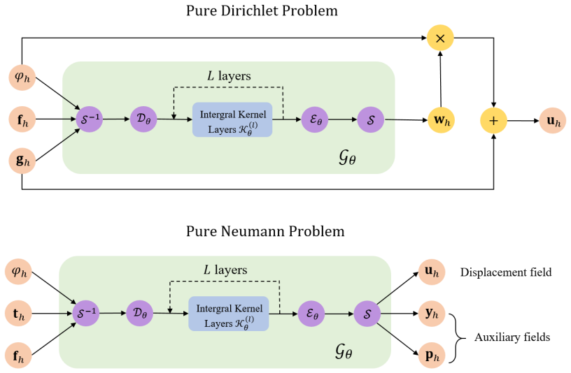
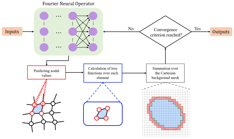
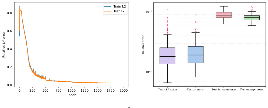
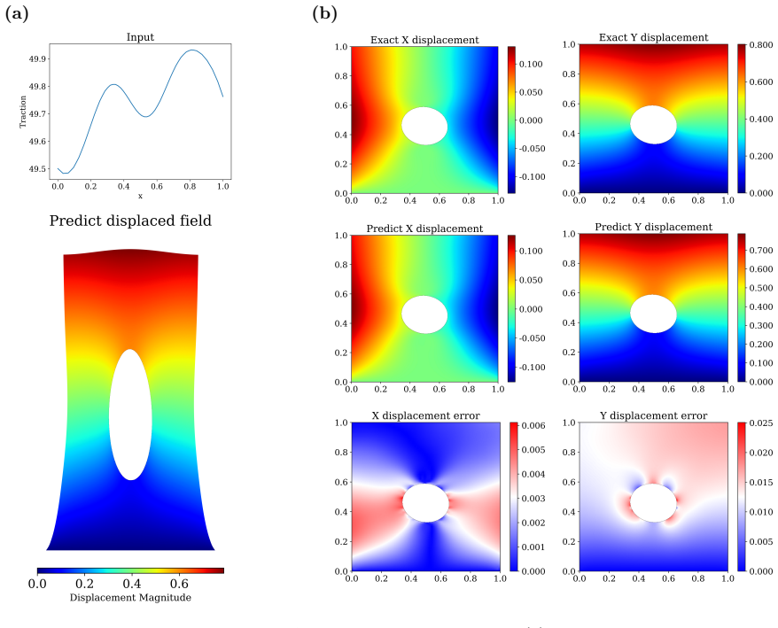
WINO establishes that the φ-FEM weak formulation itself can act as the training signal for a neural operator on variable domains. For pure Dirichlet problems, the network learns only the homogeneous lift component w_h in u_h = φ_h w_h + g_h, so boundary conditions are built into the ansatz. For traction-driven Neumann problems, the same backbone predicts the displacement together with the auxiliary fields y_h and p_h that close the unfitted weak form. Training minimizes squared nodal weak-form residuals and squared residuals of the auxiliary equations, evaluated by Gaussian quadrature on a fixed Cartesian background mesh. The resulting operator reaches relative L2 errors below 4% on all repo
What carries the argument
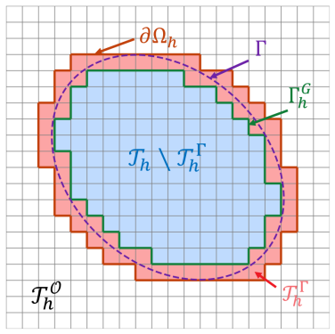
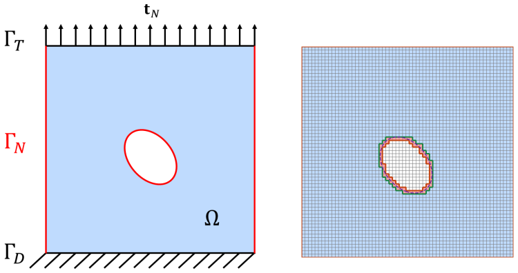
The load-bearing mechanism is the squared residual of the φ-FEM weak form, evaluated element-wise on the unchanged background mesh using Q4 and Q9 test functions. φ-FEM represents the domain implicitly through a level-set function on a Cartesian grid, avoiding body-fitted meshes and trimmed-element quadrature; the weak form handles nonsymmetric and non-energy settings where an energy-based loss would not apply. The Fourier neural operator maps input fields (level set, loads, boundary data) to either the homogeneous displacement or the displacement plus auxiliary cut-cell fields, and the loss is assembled with standard finite-element quadrature so no additional numerical differentiation in ph
Load-bearing premise
The squared weak-form residual evaluated on the background mesh, without ghost-penalty stabilization, is assumed to be a sufficient training signal: driving that loss near zero is assumed to produce the correct hyperelastic displacement rather than a spurious zero-residual mode.
What would settle it
Construct a specific load and geometry family where the φ-FEM weak form admits nontrivial zero-residual modes (for example, a cut-cell configuration with insufficient stabilization), train WINO without labels on that family, and check whether the predicted displacement matches a reference solution; if the loss is near zero but the error is large, the sufficiency assumption fails.
If this is right
- Hyperelastic operator learning no longer requires large paired datasets of converged finite-element solutions, removing the dominant data-generation bottleneck.
- Training on a fixed Cartesian background means a single WINO model can handle many geometries within one parametric family without remeshing.
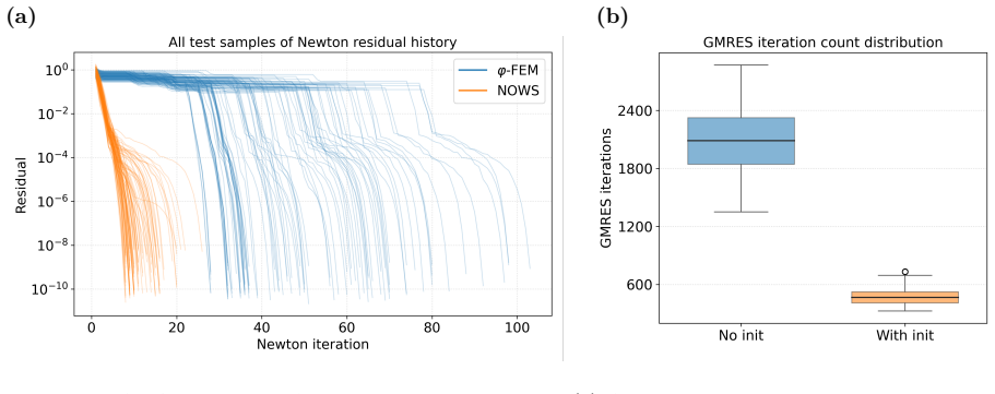
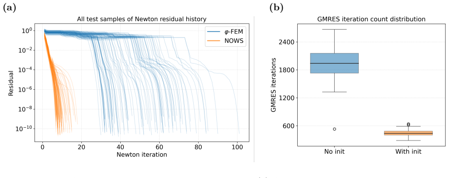
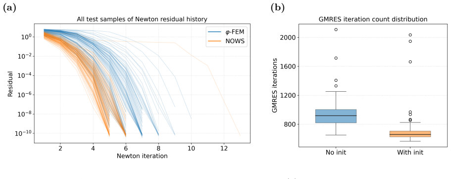
- WINO predictions provide neural-operator warm starts that reduce Newton and GMRES iteration counts, e.g., cutting nonlinear solve wall-clock time from 2.44 s to 0.47 s in the elliptical benchmark while preserving the exactness of the final finite-element solve.
- The same WINO model shows stability when evaluated on finer meshes than it was trained on, whereas a purely supervised Fourier neural operator degrades more noticeably in H1 error under such cross-resolution transfer.
- When labeled data are available, augmenting the physics loss with a supervised term further improves accuracy, giving a smooth interpolation between label-free and fully supervised regimes.
Where Pith is reading between the lines
- Editorial inference: because the method needs no energy functional, the same squared-weak-residual recipe could be transferred to other unfitted or non-variational discretizations, such as Petrov–Galerkin or stabilized cut-cell methods.
- Editorial inference: the warm-start capability suggests WINO could be embedded in optimization or inverse-design loops where many nearby loading/geometry queries must be solved repeatedly, since a 5 ms forward pass replaces several Newton iterations.
- Editorial inference: a testable extension would be to train WINO at coarse resolution and evaluate on progressively finer meshes to see whether the observed resolution invariance holds beyond the tested 51-to-256 grid range, which would strengthen the claim of mesh-independent operator learning.
Editorial analysis
A structured set of objections, weighed in public.
Referee Report
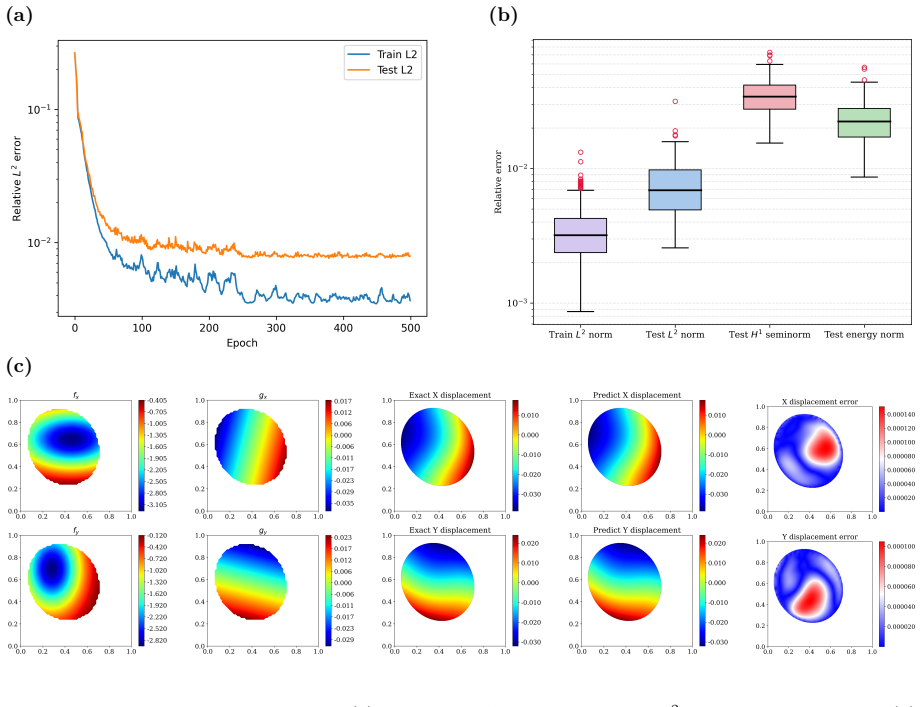
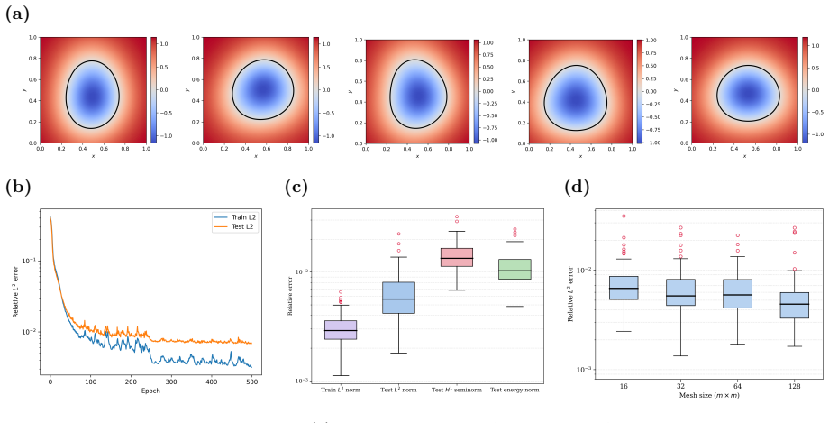
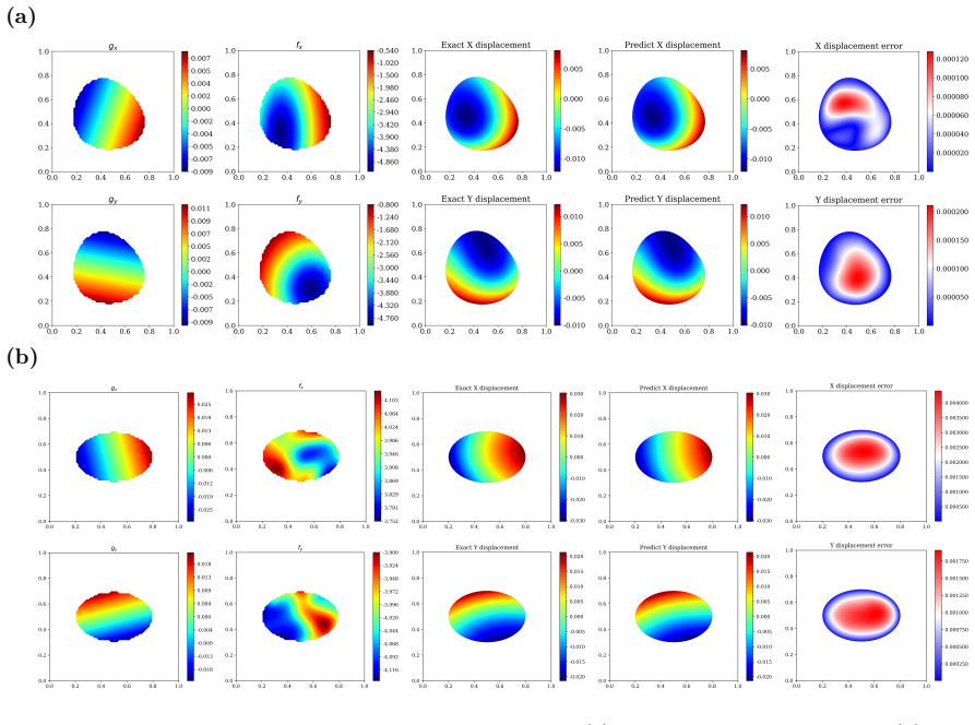
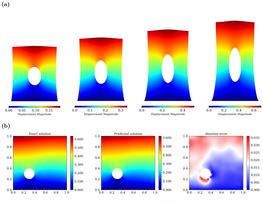
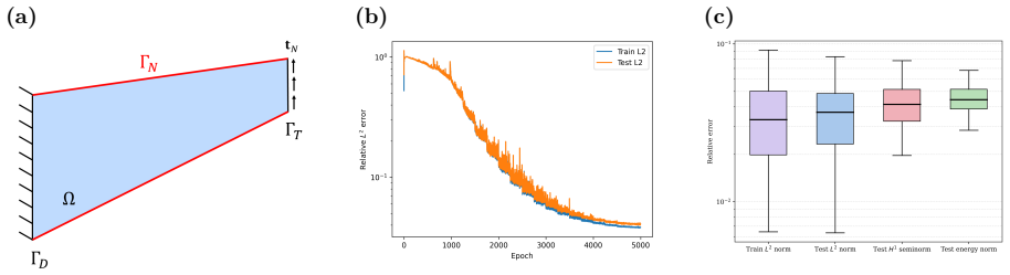
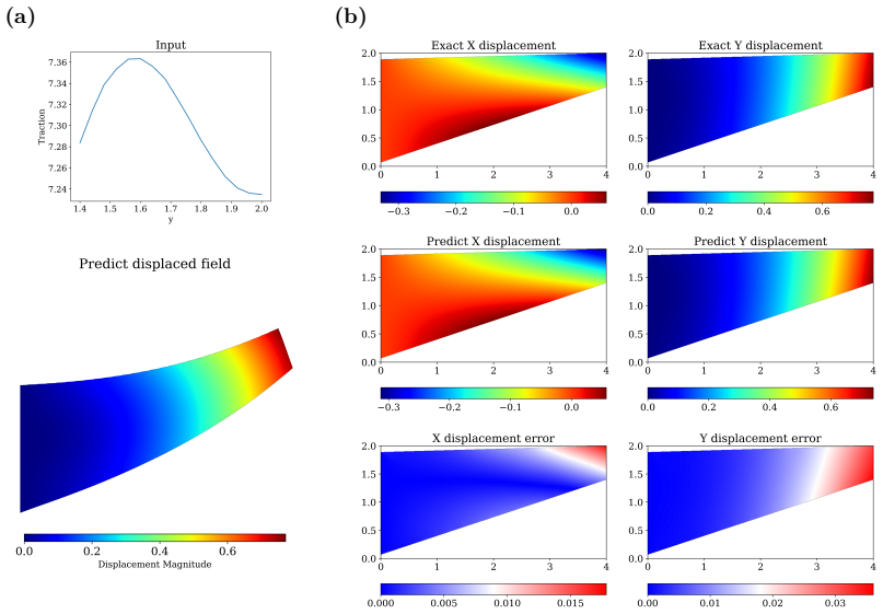
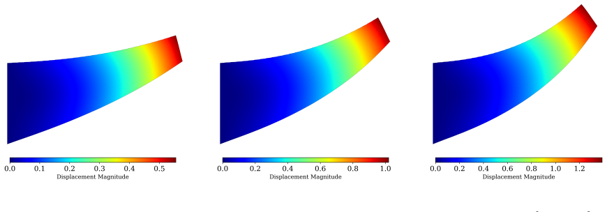
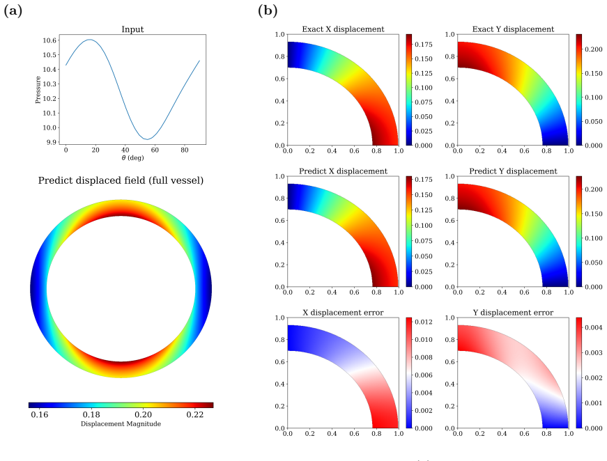
Summary. The paper proposes WINO, a weak-form physics-informed neural operator for parametric hyperelasticity on domains represented by level-set functions on a fixed Cartesian background mesh. The network is built on an FNO backbone and trained by minimizing squared φ-FEM weak-form residuals, optionally augmented by strong-form penalties for cut-cell auxiliary variables in the Neumann branch; Dirichlet conditions are imposed through the φ-FEM lift. The authors claim that this removes the need for paired reference solutions, while retaining accuracy and geometric flexibility. Five benchmark families are reported (elliptical shapes, random shapes, plate with a hole, Cook's membrane, pressure vessel), with relative L2 errors between 0.65% and 3.97%, total training times 15–70% of those of supervised FNO, and acceleration of Newton/GMRES solvers through neural-operator warm starts (NOWS).
Significance. If the central claim is valid, WINO is a useful step toward label-free operator learning for nonlinear solid mechanics on varying geometries: it avoids body-fitted remeshing, uses a weak form that aligns with finite-element practice, and produces warm starts that accelerate existing solvers. The manuscript is strong on reproducibility and breadth: code and data are publicly available, experiments include multiple error metrics, out-of-distribution tests, mesh-resolution studies, and a body-fitted convergence check for the pressure vessel. However, the core label-free assertion rests on an unproved premise — that driving the squared weak residual (2.40)/(2.42) to small values selects the physical displacement rather than a spurious zero-residual mode — and the validation partly measures self-consistency with the same φ-FEM discretization family. These issues are load-bearing and require additional analysis or targeted numerical evidence before the main claim is established.
major comments (4)
- [§2.4.2, Eqs. (2.40), (2.42); Remark 2.4] The label-free training claim rests on the squared weak residual being a sufficient training signal. Minimizing (2.40)/(2.42) only enforces a Galerkin statement against the chosen Q4/Q9 test functions; for a nonlinear hyperelastic problem with possible multiple equilibria this does not, by itself, guarantee convergence to the physical solution. Remark 2.4 explicitly drops the ghost-penalty stabilization used in the φ-FEM formulation (2.13)/(2.19), and the Neumann loss replaces the coupled system by strong-form penalties (2.38)–(2.39). No null-space check, coercivity/inf-sup argument, or branch-selection experiment is provided. I request either a theoretical justification or numerical evidence — e.g., residual Jacobian rank/conditioning on the test space, training from several initializations, or verification that near-zero loss implies agreement with an independent body-fitted reference
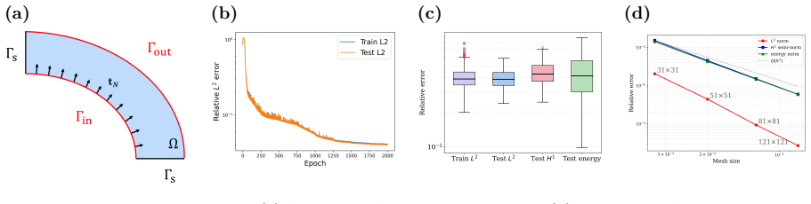
- [§3, Tables 2 and 6; Fig. 18d] Validation is partly circular: the reference solutions are produced by the same φ-FEM formulation whose residual WINO minimizes, on the same background mesh family. Only the pressure-vessel benchmark compares φ-FEM against a body-fitted FEM reference (Fig. 18d). For the other four benchmarks, a φ-FEM-consistent but physically wrong mode would not be detected by the reported errors. At least one benchmark should be re-validated against an independent body-fitted or differently discretized reference, or a subset of WINO predictions should be compared directly to body-fitted FEM solutions.
- [§3.2.1–3.2.3, Eq. (2.39); Conclusion] The auxiliary penalty weights λ1, λ2, λ3 are hand-tuned per benchmark and vary by orders of magnitude: plate with a hole uses 10−6, 10−7; Cook's membrane uses 10−7, 10−2, 1; the pressure vessel uses 10−2, 10−3. The Conclusion concedes that training is sensitive to these parameters. Because Lsq is an integral part of the label-free loss (2.40), this tuning burden weakens the practical claim that WINO avoids expensive labeled data. Please provide a systematic selection rule, a sensitivity study, or an adaptive strategy for these weights.
- [§3.1.2, Table 1] The reported training hyperparameters are internally inconsistent: the text states that the random-shape model is trained with a learning rate of 0.05, while Table 1 lists 0.005. This needs correction. In addition, the cost comparisons would be more informative if they separated data-generation time from training time; in Table 6, WINO's training time (19,242 s) is actually larger than FNO's training time (12,757 s), and the total-time advantage comes solely from saved data generation. The abstract's phrasing 'total training times of about 15%–70%' should be made consistent with the later phrasing 'total computational time by 50–80%', and the distinction between training time and total cost should be stated unambiguously.
minor comments (5)
- [Abstract and §1] There are typographical issues throughout: 'operater', 'efficiency', 'more simpler', 'A veraged'. The abstract's two percentage claims ('15%–70%' vs '50–80%') should be reconciled.
- [Table 2] The 'data generation + training time' format is unclear for WINO entries such as '0.3 + 1248.8 s': what does 0.3 s represent? Clarify the columns and units.
- [§3.1.2, Eq. (3.9)–(3.10)] The definition of φ from φg is ambiguous: the term max_{Ω} φg depends on the continuous domain and should be stated more precisely, e.g., as a nodal maximum on the background mesh.
- [§2.2, Eq. (2.14)] The notation ⟦·⟧ for the jump is defined only in the text after Eq. (2.20); please define it at first use in Eq. (2.14).
- [§3.2.2 and §3.2.3] For the Cook's membrane and pressure vessel benchmarks, the text mentions that GMRES did not converge and LU was used; the NOWS comparisons are not reported for these cases. State explicitly that the warm-start benefit was not demonstrated for these more strongly nonlinear benchmarks.
Circularity Check
No significant circularity: WINO's residual-based loss is not fitted to reference outputs, and validation includes an external body-fitted FEM convergence check.
full rationale
WINO's central training objective is Ltotal = Lweak + Lsq (Eqs. 2.36–2.40), a squared residual of the φ-FEM weak form and the cut-cell auxiliary constraints. This is the intended definition of a physics-informed solver, not a reduction of the prediction to its inputs: the loss is evaluated on level-set fields and loads, not on the reference displacement, and no fitted parameter is renamed as a predicted output. Reported errors are measured against φ-FEM reference solutions, and in the pressure-vessel case the φ-FEM reference is itself validated against a body-fitted FEM solution with convergence shown in Fig. 18d, providing external support. The self-citations ([14] for Q9 shape functions, [16]/[17] for NOWS) supply implementation details and a general warm-start strategy; neither is load-bearing for the label-free claim. The hand-tuned penalty parameters and the absence of a null-space/uniqueness analysis are correctness risks, not circularity. No equation is defined in terms of the predicted field, and no load-bearing step reduces by construction to its own inputs.
Axiom & Free-Parameter Ledger
free parameters (3)
- penalty weights λ1, λ2, λ3 =
Per benchmark: plate 1e-6/1e-7/1e-6; Cook 1e-7/1e-2/1; pressure vessel 1e-2/1e-3/1e-2
- FNO architecture and optimizer hyperparameters =
16 Fourier modes, 4 layers, width 32, batch size 50, per-case learning rate/decay/patience
- φ-FEM stabilization and reference-solver parameters =
Not fully reported (σ_D, σ_N; some Newton/GMRES tolerances are given)
axioms (5)
- domain assumption The φ-FEM weak formulations (2.13) and (2.19) are stable and coercive for the benchmark geometries and chosen stabilization parameters.
- ad hoc to paper A network that drives the squared weak residual (2.40)/(2.42) to small values yields the physically correct displacement, i.e., the residual has no spurious near-null modes on the finite test space.
- ad hoc to paper Ghost-penalty stabilization can be omitted from the WINO loss because neural fields are smooth on the background mesh.
- standard math Q4/Q9 interpolation of network nodal outputs is accurate enough for residual quadrature on active and cut cells.
- domain assumption Random sampling of level sets, loads, and body forces defines a distribution covering the test and OOD cases.
read the original abstract
We propose a Weak-form Physics-Informed Neural Operator (WINO), a data-free framework that combines the efficiency of neural operators with the geometric flexibility of the $\varphi$-finite element method ($\varphi$-FEM). $\varphi$-FEM is an unfitted method that accommodates geometric variations without body-fitted meshes, where the domain geometry is represented by the level-set function $\varphi$. To impose the boundary conditions, Dirichlet problems adopt the $\varphi$-FEM lifting so only the homogeneous displacement contribution is learned, whereas traction-driven Neumann problems additionally predict the auxiliary fields necessary for the unfitted weak formulation. Parameters are trained by minimizing squared weak-form residuals aligned with $\varphi$-FEM together with squared penalties on the cut-cell auxiliary equations, which removes the need for large paired datasets of converged reference solutions. When labeled reference data are available, an optional data-augmented variant (WINO+data) can further combine this physics-informed loss with a supervised term. After training, WINO outputs can seed the nonlinear $\varphi$-FEM solvers as neural operator warm starts (NOWS), which reduce iteration counts relative to traditional cold-started solvers. Numerical benchmarks show substantial accuracy of WINO together with total training times of about 15%-70% of those of supervised $\varphi$-FEM-FNO across all cases, without requiring reference-solution generation.
Figures
Forward citations
Cited by 1 Pith paper
-
Data-free neural PDE solvers based on Graph Neural Networks and weak forms
A graph-neural-network PDE solver trained on the weak-form force residual — no simulation data — reports residual convergence below 1% on unseen load cases and one modified geometry, with residual-based test-time refinement.
Reference graph
Works this paper leans on
-
[1]
Nonlinear solid mechanics: a continuum approach for engineering science,
G. A. Holzapfel, “Nonlinear solid mechanics: a continuum approach for engineering science,” 2002
2002
-
[2]
Topics in finite elasticity: hyperelasticity of rubber, elastomers, and biological tissues— with examples,
M. F. Beatty, “Topics in finite elasticity: hyperelasticity of rubber, elastomers, and biological tissues— with examples,” 1987
1987
-
[3]
O. C. Zienkiewicz, R. L. Taylor, P. Nithiarasu, and J. Zhu, The finite element method . Elsevier, 1977, vol. 3
1977
-
[4]
An introduction to the finite element method,
J. N. Reddy, “An introduction to the finite element method,” in Dynamics of Earth’s Fluid System . CRC Press, 2026, pp. 199–226
2026
-
[5]
Finite element implementation of incompressible, transversely isotropic hyperelasticity,
J. A. Weiss, B. N. Maker, and S. Govindjee, “Finite element implementation of incompressible, transversely isotropic hyperelasticity,” Computer methods in applied mechanics and engineering , vol. 135, no. 1-2, pp. 107–128, 1996
1996
-
[6]
J. W. Thomas, Numerical partial differential equations: finite difference methods . Springer Science & Business Media, 2013, vol. 22
2013
-
[7]
L. Lu, P. Jin, and G. E. Karniadakis, “Deeponet: Learning nonlinear operators for identifying differential equations based on the universal approximation theorem of operators,” arXiv preprint arXiv:1910.03193, 2019
Pith/arXiv arXiv 1910
-
[8]
Learning nonlinear operators via deeponet based on the universal approximation theorem of operators,
L. Lu, P. Jin, G. Pang, Z. Zhang, and G. E. Karniadakis, “Learning nonlinear operators via deeponet based on the universal approximation theorem of operators,” Nature machine intelligence , vol. 3, no. 3, pp. 218–229, 2021
2021
-
[9]
Fourier neural operator for parametric partial differential equations,
Z. Li, N. Kovachki, K. Azizzadenesheli, B. Liu, K. Bhattacharya, A. Stuart, and A. Anand- kumar, “Fourier neural operator for parametric partial differential equations,” arXiv preprint arXiv:2010.08895, 2020
Pith/arXiv arXiv 2010
-
[10]
Synergistic learning with multi-task deeponet for efficient pde problem solving,
V. Kumar, S. Goswami, K. Kontolati, M. D. Shields, and G. E. Karniadakis, “Synergistic learning with multi-task deeponet for efficient pde problem solving,” Neural Networks , vol. 184, p. 107113, 2025. 37
2025
-
[11]
Physics-informed neural operator for learning partial differential equations,
Z. Li, H. Zheng, N. Kovachki, D. Jin, H. Chen, B. Liu, K. Azizzadenesheli, and A. Anandkumar, “Physics-informed neural operator for learning partial differential equations,” ACM/IMS Journal of Data Science , vol. 1, no. 3, pp. 1–27, 2024
2024
-
[12]
Learning the solution operator of parametric partial dif- ferential equations with physics-informed deeponets,
S. Wang, H. Wang, and P. Perdikaris, “Learning the solution operator of parametric partial dif- ferential equations with physics-informed deeponets,” Science advances, vol. 7, no. 40, p. eabi8605, 2021
2021
-
[13]
Physics-informed machine learning in biomedical science and engineering,
N. Ahmadi, Q. Cao, J. D. Humphrey, and G. E. Karniadakis, “Physics-informed machine learning in biomedical science and engineering,” Annual Review of Biomedical Engineering , vol. 28, no. 1, pp. 309–336, 2026
2026
-
[14]
Variational physics-informed neural operator (vino) for solving partial differential equations,
M. S. Eshaghi, C. Anitescu, M. Thombre, Y. Wang, X. Zhuang, and T. Rabczuk, “Variational physics-informed neural operator (vino) for solving partial differential equations,” Computer Methods in Applied Mechanics and Engineering , vol. 437, p. 117785, 2025
2025
-
[15]
Finite element operator network for solving parametric pdes,
J. Y. Lee, S. Ko, and Y. Hong, “Finite element operator network for solving parametric pdes,” arXiv preprint arXiv:2308.04690 , 2023
Pith/arXiv arXiv 2023
-
[16]
Nows: Neural operator warm starts for accelerating iterative solvers,
M. S. Eshaghi, C. Anitescu, N. Valizadeh, Y. Wang, X. Zhuang, and T. Rabczuk, “Nows: Neural operator warm starts for accelerating iterative solvers,” arXiv preprint arXiv:2511.02481 , 2025
Pith/arXiv arXiv 2025
-
[17]
Y. Wang, Z. Hao, M. S. Eshaghi, C. Anitescu, X. Zhuang, T. Rabczuk, and Y. Liu, “Pretrain finite element method: A pretraining and warm-start framework for pdes via physics-informed neural operators,” arXiv preprint arXiv:2601.03086 , 2026
arXiv 2026
-
[18]
Level set methods: an overview and some recent results,
S. Osher and R. P. Fedkiw, “Level set methods: an overview and some recent results,” Journal of Computational physics , vol. 169, no. 2, pp. 463–502, 2001
2001
-
[19]
Level set methods and dynamic implicit surfaces,
S. Osher, R. Fedkiw, and K. Piechor, “Level set methods and dynamic implicit surfaces,” Appl. Mech. Rev., vol. 57, no. 3, pp. B15–B15, 2004
2004
-
[20]
ϕ-fem: a finite element method on domains defined by level-sets,
M. Duprez and A. Lozinski, “ ϕ-fem: a finite element method on domains defined by level-sets,” SIAM Journal on Numerical Analysis , vol. 58, no. 2, pp. 1008–1028, 2020
2020
-
[21]
φ-fem, a finite element method on domains defined by level-sets: the neumann boundary case,
M. Duprez, V. Lleras, and A. Lozinski, “ φ-fem, a finite element method on domains defined by level-sets: the neumann boundary case,” 2020
2020
-
[22]
φ-fem-fno: a new approach to train a neural operator as a fast pde solver for variable geometries,
M. Duprez, V. Lleras, A. Lozinski, V. Vigon, and K. Vuillemot, “ φ-fem-fno: a new approach to train a neural operator as a fast pde solver for variable geometries,” Communications in Nonlinear Science and Numerical Simulation , p. 109131, 2025
2025
-
[23]
Cut finite element methods,
E. Burman, P. Hansbo, M. G. Larson, and S. Zahedi, “Cut finite element methods,” Acta Numerica, vol. 34, pp. 1–121, 2025
2025
-
[24]
Bonet and R
J. Bonet and R. D. Wood, Nonlinear continuum mechanics for finite element analysis . Cambridge university press, 1997
1997
-
[25]
C. T. Kelley, Solving nonlinear equations with Newton ’s method . SIAM, 2003
2003
-
[26]
Nitsol: A newton iterative solver for nonlinear systems,
M. Pernice and H. F. Walker, “Nitsol: A newton iterative solver for nonlinear systems,” SIAM Journal on Scientific Computing , vol. 19, no. 1, pp. 302–318, 1998. 38
1998
-
[27]
Function minimization by conjugate gradients,
R. Fletcher and C. M. Reeves, “Function minimization by conjugate gradients,” The computer journal, vol. 7, no. 2, pp. 149–154, 1964
1964
-
[28]
A survey of nonlinear conjugate gradient methods,
W. W. Hager and H. Zhang, “A survey of nonlinear conjugate gradient methods,” Pacific journal of Optimization, vol. 2, no. 1, pp. 35–58, 2006
2006
-
[29]
Gmres: A generalized minimal residual algorithm for solving non- symmetric linear systems,
Y. Saad and M. H. Schultz, “Gmres: A generalized minimal residual algorithm for solving non- symmetric linear systems,” SIAM Journal on scientific and statistical computing , vol. 7, no. 3, pp. 856–869, 1986
1986
-
[30]
Gmres with deflated restarting,
R. B. Morgan, “Gmres with deflated restarting,” SIAM Journal on Scientific Computing , vol. 24, no. 1, pp. 20–37, 2002
2002
-
[31]
Petsc users manual,
S. Balay, S. Abhyankar, M. Adams, J. Brown, P. Brune, K. Buschelman, L. Dalcin, A. Dener, V. Eijkhout, W. Gropp et al. , “Petsc users manual,” 2019
2019
-
[32]
Soap: Improving and stabilizing shampoo using adam,
N. Vyas, D. Morwani, R. Zhao, M. Kwun, I. Shapira, D. Brandfonbrener, L. Janson, and S. Kakade, “Soap: Improving and stabilizing shampoo using adam,” arXiv preprint arXiv:2409.11321 , 2024
Pith/arXiv arXiv 2024
-
[33]
Gaussian processes in machine learning,
C. E. Rasmussen, “Gaussian processes in machine learning,” in Summer school on machine learning . Springer, 2003, pp. 63–71
2003
-
[34]
G. H. Golub and C. F. Van Loan, Matrix computations . JHU press, 2013. 39
2013
discussion (0)
Sign in with ORCID, Apple, or X to comment. Anyone can read and Pith papers without signing in.