Continuous-time quantum control across an exponentially small bottleneck in a frustrated Ising ring model
Pith reviewed 2026-06-27 22:05 UTC · model grok-4.3
The pith
Optimized continuous-time schedules prepare ground states in linear time despite an exponentially small gap in a frustrated Ising ring.
A machine-rendered reading of the paper's core claim, the machinery that carries it, and where it could break.
Core claim
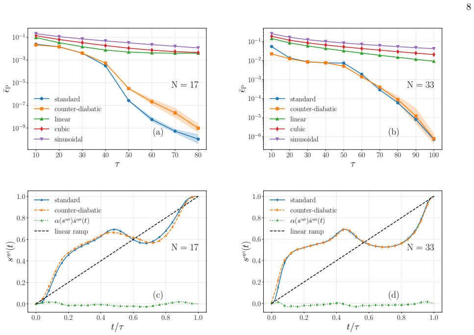
In the frustrated Ising ring, continuous-time quantum control via optimized smooth schedules allows the system to bypass the exponentially small gap through nonadiabatic transitions, achieving ground-state preparation with annealing times that scale linearly with system size for a fixed residual energy, outperforming both linear schedules and variational counter-diabatic corrections.
What carries the argument
Dressed-CRAB optimization of the annealing schedule, using digitized dynamics to compute gradients, which discovers nonadiabatic paths that avoid the minimum gap bottleneck.
If this is right
- The annealing time required to reach a fixed residual-energy threshold grows linearly with system size.
- The exponentially small minimum gap can be bypassed via strongly nonadiabatic dynamics.
- A lowest-order variational counter-diabatic correction yields no improvement once the schedule is optimized.
- Ground-state preparation remains possible in linear time even when adiabaticity cannot be maintained.
Where Pith is reading between the lines
- Similar schedule optimization may apply to other many-body models limited by small gaps.
- The linear scaling could reduce the total evolution time needed for practical ground-state preparation in larger rings.
- The nonadiabatic bypass mechanism might generalize beyond this specific frustrated ring geometry.
Load-bearing premise
The dressed-CRAB optimization combined with digitized dynamics reliably discovers nonadiabatic schedules that achieve the linear scaling without hidden costs or model-specific artifacts.
What would settle it
Numerical checks on larger system sizes showing that the time to reach the fixed residual-energy threshold still grows exponentially with ring size would falsify the linear scaling result.
Figures
read the original abstract
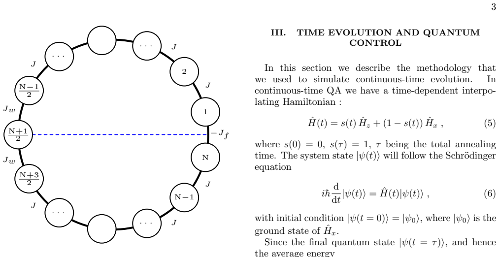
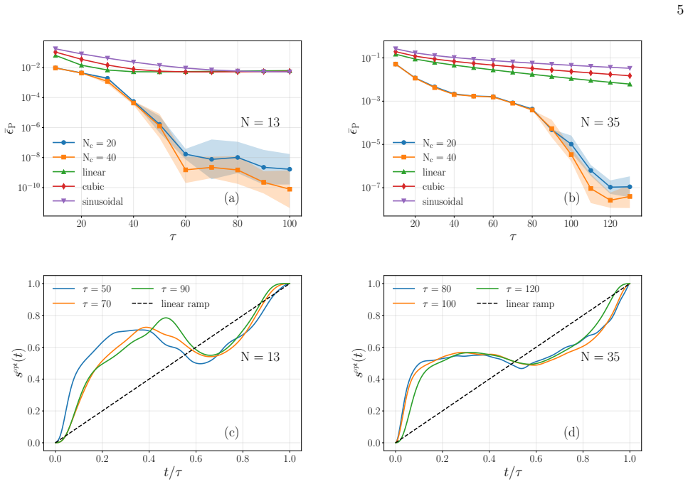
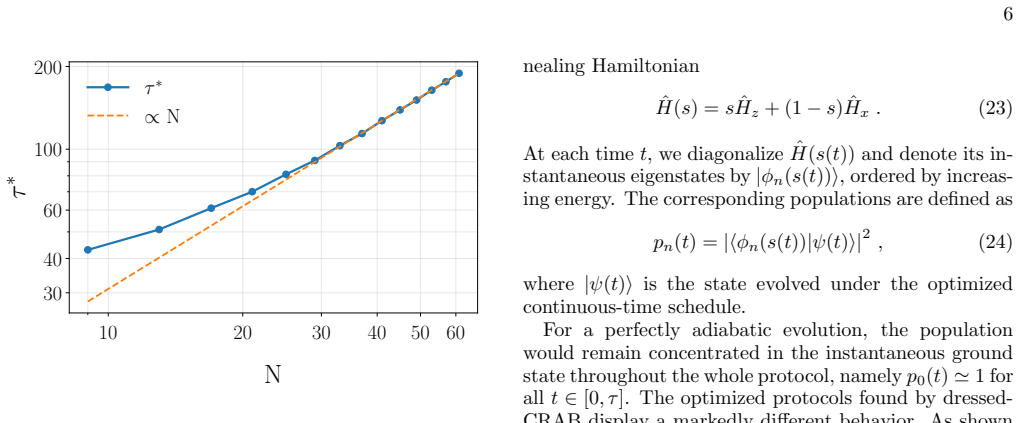
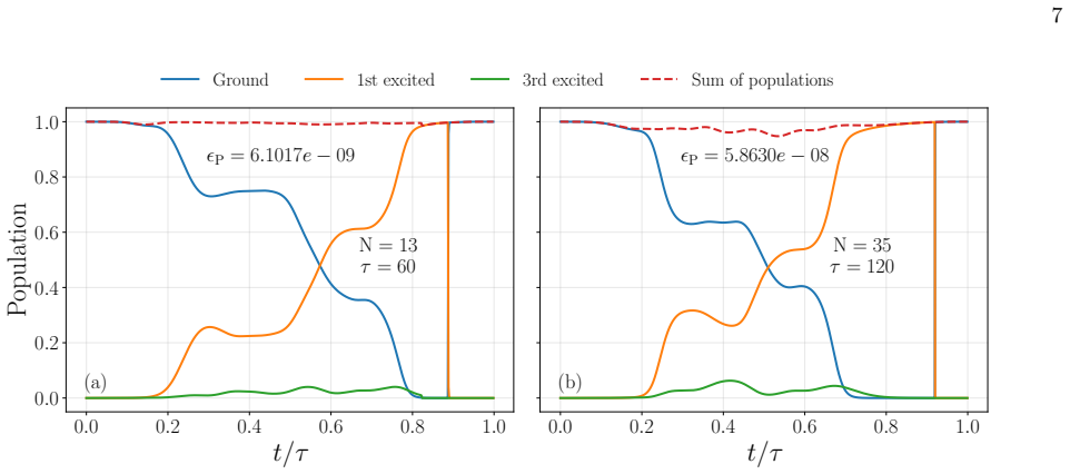
Continuous-time Quantum Annealing (QA) is a strategy for preparing the ground state of nontrivial many-body systems. In its standard form, the dynamics is generated by a time-dependent interpolation between a simple driving Hamiltonian and the target problem Hamiltonian, usually implemented through a linear schedule. This approach faces the crucial bottleneck of small spectral gaps, which may require exponentially long annealing times to ensure adiabaticity. Here, we show how to implement quantum control over the annealing schedule in a frustrated Ising ring, one of the simplest models exhibiting an exponentially small bottleneck gap. By optimizing smooth continuous-time annealing schedules with a dressed-CRAB approach, and using a digitized representation of the dynamics to efficiently evaluate gradients, we construct protocols that strongly outperform standard fixed schedules. The optimized dynamics bypasses the bottleneck through a strongly nonadiabatic mechanism, leading to efficient ground-state preparation despite the exponentially small minimum gap. In particular, the annealing time required to reach a fixed residual-energy threshold is found to grow linearly with system size rather than exponentially. We further examine a lowest-order variational counter-diabatic correction and find that, once schedule optimization is allowed, it does not lead to any improvement.
Editorial analysis
A structured set of objections, weighed in public.
Referee Report
Summary. The paper claims that in a frustrated Ising ring model with an exponentially small bottleneck gap, dressed-CRAB optimization of smooth continuous-time annealing schedules (using a digitized representation of the dynamics to evaluate gradients) produces nonadiabatic protocols that achieve linear-in-N scaling of the annealing time to a fixed residual-energy threshold, thereby bypassing the gap. It further reports that a lowest-order variational counter-diabatic correction yields no additional improvement once schedule optimization is permitted.
Significance. If the central claim holds under exact continuous-time evolution, the result would demonstrate that nonadiabatic quantum control can convert an exponential bottleneck into linear scaling for ground-state preparation in a minimal model exhibiting a closing gap. This would strengthen the case for schedule optimization in quantum annealing beyond adiabaticity and provide a concrete benchmark for counter-diabatic methods. The explicit comparison of optimized schedules against both linear annealing and variational counter-diabatic driving is a positive feature.
major comments (2)
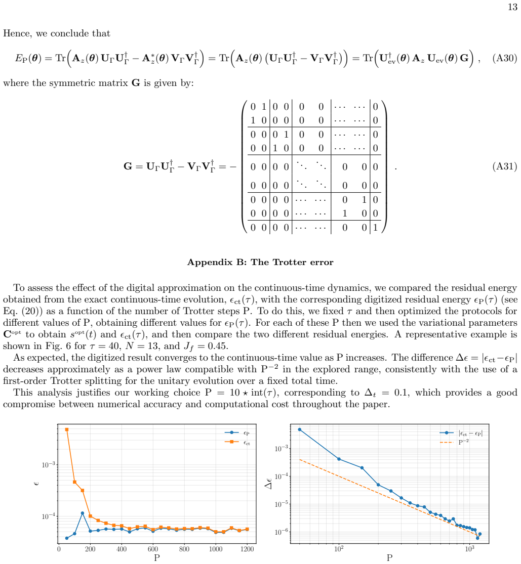
- [Methods (gradient evaluation via digitized dynamics)] The central claim of linear scaling in continuous time rests on protocols discovered via gradients computed in a digitized representation of the dynamics. The manuscript should include an explicit convergence study (e.g., residual energy versus digitization step size δt o 0 at fixed optimized schedule) to rule out the possibility that performance depends on discretization artifacts rather than the underlying continuous Hamiltonian. Without this, the reported linear scaling cannot be taken as established for the continuous-time model.
- [Results (scaling plots)] The linear scaling is asserted for a fixed residual-energy threshold across system sizes. The manuscript must report the precise threshold value, the range of N examined, the number of independent optimization runs, and error bars or worst-case residuals to substantiate that the scaling is not an artifact of a particular threshold or finite-N window.
minor comments (2)
- [Methods] Notation for the dressed-CRAB parameters and the precise form of the digitized Trotter or Suzuki-Trotter decomposition used for gradient evaluation should be stated explicitly in the main text rather than deferred to supplementary material.
- [Figures] Figure captions for the scaling plots should state the exact residual-energy threshold and the definition of annealing time used.
Simulated Author's Rebuttal
We thank the referee for their positive assessment of the work's potential significance and for the detailed, constructive major comments. We address each point below and will revise the manuscript to incorporate the requested clarifications and analyses.
read point-by-point responses
-
Referee: [Methods (gradient evaluation via digitized dynamics)] The central claim of linear scaling in continuous time rests on protocols discovered via gradients computed in a digitized representation of the dynamics. The manuscript should include an explicit convergence study (e.g., residual energy versus digitization step size δt → 0 at fixed optimized schedule) to rule out the possibility that performance depends on discretization artifacts rather than the underlying continuous Hamiltonian. Without this, the reported linear scaling cannot be taken as established for the continuous-time model.
Authors: We agree that an explicit convergence study is required to establish that the reported performance holds in the continuous-time limit. In the revised manuscript we will add a dedicated subsection (or appendix) presenting residual energy versus digitization step size δt for representative optimized schedules at fixed N, demonstrating convergence as δt → 0. This will confirm that the linear scaling is not an artifact of the digitized gradient evaluation. revision: yes
-
Referee: [Results (scaling plots)] The linear scaling is asserted for a fixed residual-energy threshold across system sizes. The manuscript must report the precise threshold value, the range of N examined, the number of independent optimization runs, and error bars or worst-case residuals to substantiate that the scaling is not an artifact of a particular threshold or finite-N window.
Authors: We will update the manuscript (both main text and figure captions) to state explicitly the residual-energy threshold employed, the precise range of system sizes N studied, the number of independent optimization runs performed per N, and to include error bars (or worst-case residuals) on the scaling data. These additions will allow readers to assess the robustness of the linear scaling claim. revision: yes
Circularity Check
No circularity: numerical optimization results are independent of inputs
full rationale
The paper reports outcomes of numerical optimization (dressed-CRAB schedules with digitized gradient evaluation) applied to a frustrated Ising ring. The central finding—that annealing time to fixed residual energy scales linearly with N—is presented as an empirical result of running the optimizer, not as a quantity fitted or defined in terms of itself. No self-definitional steps, fitted-input predictions, or load-bearing self-citations appear in the abstract or described method; the digitized dynamics serve as a computational tool rather than a definitional reduction. The derivation chain is therefore self-contained against external benchmarks (numerical simulation of the continuous-time model).
Axiom & Free-Parameter Ledger
Forward citations
Cited by 1 Pith paper
-
Pauli-Sparse regularised Counterdiabatic Shortcuts for Linear-Ramp QAOA
A regularized Pauli-sparse counterdiabatic method is added to linear-ramp QAOA, yielding higher approximation ratios on ferromagnetic chain and perturbed MaxCut instances than the uncorrected ramp.
Reference graph
Works this paper leans on
-
[1]
(A10) and (A11), the variousU p
(A17) where, forp= 1,· · ·,P: Up(θx p , θz p) = e−2iθx p Hxe−2iθz p Hz .(A18) Notice that, due to the block form ofH x/z, see Eqs. (A10) and (A11), the variousU p. In particular, the various exponentials can be calculated analytically, using e−2iθx p Ax = cos(2hθx p)isin(2hθ x p) 0 0 · · · · · · 0 isin(2hθ x p) cos(2hθ x p) 0 0 · · · · · ·...
-
[2]
A. B. Finnila, M. A. Gomez, C. Sebenik, C. Stenson, and J. D. Doll, Chemical Physics Letters219, 343 (1994), ISSN 0009-2614
1994
-
[3]
Kadowaki and H
T. Kadowaki and H. Nishimori, Physical Review E58, 5355 (1998)
1998
-
[4]
G. E. Santoro, R. Martonak, E. Tosatti, and R. Car, Science295, 2427 (2002)
2002
-
[5]
G. E. Santoro and E. Tosatti, Journal of Physics A: Mathematical and General39, R393 (2006)
2006
-
[6]
Albash and D
T. Albash and D. A. Lidar, Rev. Mod. Phys.90, 015002 16 (2018)
2018
-
[7]
Caneva, R
T. Caneva, R. Fazio, and G. E. Santoro, Phys. Rev. B 76, 144427 (2007)
2007
-
[8]
Knysh, Nature Communications7, 12370 (2016)
S. Knysh, Nature Communications7, 12370 (2016)
2016
-
[9]
Roberts, L
D. Roberts, L. Cincio, A. Saxena, A. Petukhov, and S. Knysh, Phys. Rev. A101, 042317 (2020)
2020
-
[10]
Bapst, L
V. Bapst, L. Foini, F. Krzakala, G. Semerjian, and F. Zamponi, Phys. Rep.523, 127 (2013)
2013
-
[11]
Matsuura, S
S. Matsuura, S. Buck, V. Senicourt, and A. Zaribafiyan, Phys. Rev. A103, 052435 (2021)
2021
-
[12]
Cˆ ot´ e, F
J. Cˆ ot´ e, F. Sauvage, M. Larocca, M. Jonsson, L. Cin- cio, and T. Albash, Quantum Science and Technology8, 045033 (2023)
2023
-
[13]
Quiroz, Phys
G. Quiroz, Phys. Rev. A99, 062306 (2019)
2019
-
[14]
P. R. Hegde, G. Passarelli, A. Scocco, and P. Lucignano, Phys. Rev. A105, 012612 (2022)
2022
-
[15]
Passarelli, V
G. Passarelli, V. Cataudella, and P. Lucignano, Phys. Rev. B100, 024302 (2019)
2019
-
[16]
Caneva, T
T. Caneva, T. Calarco, and S. Montangero, Phys. Rev. A84, 022326 (2011)
2011
-
[17]
N. Rach, M. M. M¨ uller, T. Calarco, and S. Montangero, Phys. Rev. A92, 062343 (2015)
2015
-
[18]
M. V. Berry, Journal of Physics A: Mathematical and Theoretical42, 365303 (2009)
2009
-
[19]
Kolodrubetz, D
M. Kolodrubetz, D. Sels, P. Mehta, and A. Polkovnikov, Physics Reports697, 1 (2017), ISSN 0370-1573
2017
-
[20]
Gu´ ery-Odelin, A
D. Gu´ ery-Odelin, A. Ruschhaupt, A. Kiely, E. Tor- rontegui, S. Mart´ ınez-Garaot, and J. G. Muga, Rev. Mod. Phys.91, 045001 (2019)
2019
-
[21]
Torrontegui, S
E. Torrontegui, S. Ib´ a˜ nez, S. Mart´ ınez-Garaot, M. Mod- ugno, A. del Campo, D. Gu´ ery-Odelin, A. Ruschhaupt, X. Chen, and J. G. Muga, inAdvances in Atomic, Molec- ular, and Optical Physics, edited by E. Arimondo, P. R. Berman, and C. C. Lin (Academic Press, 2013), vol. 62 ofAdvances In Atomic, Molecular, and Optical Physics, pp. 117–169
2013
-
[22]
E. Farhi, J. Goldstone, and S. Gutmann,A quan- tum approximate optimization algorithm(2014), arXiv:1411.4028
Pith/arXiv arXiv 2014
-
[23]
N. N. Hegade, X. Chen, and E. Solano, Phys. Rev. Res. 4, L042030 (2022)
2022
-
[24]
Chandarana, N
P. Chandarana, N. N. Hegade, K. Paul, F. Albarr´ an- Arriagada, E. Solano, A. del Campo, and X. Chen, Phys. Rev. Res.4, 013141 (2022)
2022
-
[25]
ˇCepait˙ e, A
I. ˇCepait˙ e, A. Polkovnikov, A. J. Daley, and C. W. Dun- can, PRX Quantum4, 010312 (2023)
2023
-
[26]
R. Wang, V. R. Arezzo, K. Thengil, G. Pecci, and G. E. Santoro, Quantum Sci. Technol.10, 035052 (2025)
2025
-
[27]
Grabarits, F
A. Grabarits, F. Balducci, and A. del Campo, PRX Quantum7, 010322 (2026)
2026
-
[28]
Jordan and E
P. Jordan and E. Wigner, Zeitschrift f¨ ur Physik47, 631 (1928), ISSN 0044-3328
1928
-
[29]
G. B. Mbeng, A. Russomanno, and G. E. Santoro, Sci- Post Physics Lecture Notes82(2024)
2024
-
[30]
V. R. Arezzo, R. Wang, K. Thengil, G. Pecci, and G. E. Santoro, Phys. Rev. A113, 012610 (2026)
2026
-
[31]
Thengil, V
K. Thengil, V. R. Arezzo, and G. E. Santoro, In prepa- ration (2026)
2026
-
[32]
Doria, T
P. Doria, T. Calarco, and S. Montangero, Phys. Rev. Lett.106, 190501 (2011)
2011
-
[33]
C. P. Koch, U. Boscain, T. Calarco, G. Dirr, S. Fil- ipp, S. J. Glaser, R. Kosloff, S. Montangero, T. Schulte- Herbr¨ uggen, D. Sugny, et al., EPJ Quantum Technology 9, 19 (2022)
2022
-
[34]
Morita and H
S. Morita and H. Nishimori, Journal of Mathematical Physics49, 125210 (2008), ISSN 0022-2488
2008
-
[35]
Barends, A
R. Barends, A. Shabani, L. Lamata, J. Kelly, A. Mezza- capo, U. L. Heras, R. Babbush, A. G. Fowler, B. Camp- bell, Y. Chen, et al., Nature534, 222 (2016)
2016
-
[36]
G. B. Mbeng, L. Arceci, and G. E. Santoro, Phys. Rev. B100, 224201 (2019)
2019
-
[37]
G. B. Mbeng, R. Fazio, and G. Santoro,Quantum Annealing: a journey through Digitalization, Control, and hybrid Quantum Variational schemes(2019), arXiv: 1906.08948
arXiv 2019
-
[38]
Pecci, R
G. Pecci, R. Wang, P. Torta, G. B. Mbeng, and G. San- toro, Quantum Sci. Technol.9, 045013 (2024), ISSN 2058-9565
2024
-
[39]
Nocedal and S
J. Nocedal and S. J. Wright,Numerical optimization (Springer, 1999)
1999
-
[40]
L. T. Brady, C. L. Baldwin, A. Bapat, Y. Kharkov, and A. V. Gorshkov, Phys. Rev. Lett.126, 070505 (2021)
2021
-
[41]
V. R. Arezzo and G. E. Santoro (2026), (in preparation)
2026
-
[42]
Rossmann,Lie Groups: An Introduction Through Linear Groups, Oxford Mathematics (Oxford University Press, 2006), ISBN 9780199202515
W. Rossmann,Lie Groups: An Introduction Through Linear Groups, Oxford Mathematics (Oxford University Press, 2006), ISBN 9780199202515
2006
-
[43]
Wurtz and P
J. Wurtz and P. J. Love, Quantum6, 635 (2022), ISSN 2521-327X
2022
-
[44]
G. Lami, P. Torta, G. E. Santoro, and M. Collura, Sci- Post Phys.14, 117 (2023)
2023
-
[45]
Collura, G
M. Collura, G. Lami, N. Ranabhat, and A. Santini, Tensor Network Techniques for Quantum Computation (OAPEN, 2025)
2025
-
[46]
It should not be understood as assuming that the residual energiesϵ (r) P (τ) are exactly log-normally distributed
This is a natural choice for positive quantities spanning several orders of magnitude. It should not be understood as assuming that the residual energiesϵ (r) P (τ) are exactly log-normally distributed
discussion (0)
Sign in with ORCID, Apple, or X to comment. Anyone can read and Pith papers without signing in.