Arrival times of an atomic Bose-Einstein condensate
Pith reviewed 2026-06-26 15:11 UTC · model grok-4.3
The pith
Solving the time-dependent Gross-Pitaevskii equation shows how interactions modify arrival time distributions of a Bose-Einstein condensate close to the trap.
A machine-rendered reading of the paper's core claim, the machinery that carries it, and where it could break.
Core claim
The distribution of arrival times for an interacting atomic Bose-Einstein condensate is obtained by solving the time-dependent Gross-Pitaevskii equation analytically and numerically, which modifies the predictions previously made for non-interacting particles in the close-to-trap detection regime.
What carries the argument
The time-dependent Gross-Pitaevskii equation, which evolves the condensate wave function while incorporating particle interactions.
If this is right
- The arrival time distribution acquires an explicit dependence on the interaction strength through the Gross-Pitaevskii dynamics.
- Analytical solutions yield closed-form modifications to the non-interacting arrival time formulas.
- Numerical solutions of the equation confirm the analytical results and extend them to time-dependent trapping potentials.
- The modified distribution applies only in the regime where the detector sits near the original trap location.
Where Pith is reading between the lines
- Future experiments could directly compare measured arrival statistics against these Gross-Pitaevskii results to test the mean-field approximation at short distances.
- The same framework may be extended to other detection geometries or to condensates with attractive interactions.
- Detector timing resolution requirements can be estimated from the spread of the interacting arrival time distribution.
Load-bearing premise
The time-dependent Gross-Pitaevskii equation remains an adequate description of the condensate dynamics in the close-to-trap detection regime.
What would settle it
An experimental measurement of the arrival time distribution for atoms from a Bose-Einstein condensate detected close to the trap that deviates from the analytical or numerical Gross-Pitaevskii predictions would show the mean-field description fails in this regime.
Figures



read the original abstract
The times of flight of an atomic Bose-Einstein condensate are theoretically investigated in the experimentally unexplored regime corresponding to detection close to the trap of the condensate. In this regime, there is no consensus on how to calculate the distribution of times of arrival onto the detector. For non-interacting particles, distinct theoretical predictions have been made in the past. This work analyses how these predictions are modified for an interacting Bose-Einstein condensate. For this purpose, a time-dependent Gross-Pitaevskii equation is solved analytically and numerically.
Editorial analysis
A structured set of objections, weighed in public.
Referee Report
Summary. The manuscript investigates arrival times of atoms from an interacting atomic Bose-Einstein condensate detected close to the trap, an experimentally unexplored regime lacking consensus even for non-interacting particles. It extends prior non-interacting predictions by solving the time-dependent Gross-Pitaevskii equation both analytically and numerically to determine how interactions modify the arrival-time distributions.
Significance. If the mapping from GPE solutions to observable arrival times is valid, the work would supply concrete interaction-induced modifications to existing non-interacting predictions and could guide experiments in this regime.
major comments (1)
- [Abstract] Abstract: the central claim that analytic and numeric GPE solutions demonstrate how interactions modify arrival-time predictions rests on the unexamined assumption that the mean-field wavefunction evolution yields the correct single-particle arrival-time distribution (via probability current or detector density) in the dense near-trap regime; the manuscript provides no discussion of why number fluctuations and correlations neglected by GPE can be ignored here.
Simulated Author's Rebuttal
We thank the referee for their comment on the applicability of the GPE. We address the concern below and will revise the manuscript accordingly.
read point-by-point responses
-
Referee: [Abstract] Abstract: the central claim that analytic and numeric GPE solutions demonstrate how interactions modify arrival-time predictions rests on the unexamined assumption that the mean-field wavefunction evolution yields the correct single-particle arrival-time distribution (via probability current or detector density) in the dense near-trap regime; the manuscript provides no discussion of why number fluctuations and correlations neglected by GPE can be ignored here.
Authors: We agree that the manuscript would benefit from explicit discussion of this assumption. In the revised version we will insert a paragraph (likely in the introduction) noting that for typical experimental N ≳ 10^4 the relative number fluctuations are suppressed by 1/√N and the GPE provides the leading-order description of the condensate density and phase that enter the probability current. We will also state that full many-body treatments remain computationally prohibitive for the time-dependent near-trap problem and that the GPE is the standard tool used for interacting BECs in this regime, while acknowledging that higher-order correlations could affect finer statistics and are left for future work. revision: yes
Circularity Check
No circularity: GPE solution treated as independent input to arrival-time analysis
full rationale
The paper states it solves the time-dependent Gross-Pitaevskii equation analytically and numerically to examine how non-interacting arrival-time predictions change under interactions. No quoted step shows a derived distribution or prediction reducing by construction to a fitted parameter, self-citation, or renamed input. The central mapping from GPE wavefunction to arrival-time statistics is presented as a direct computation rather than a tautology. External validity of the mean-field model in the near-trap regime is a separate modeling assumption, not a circularity in the derivation chain itself.
Axiom & Free-Parameter Ledger
axioms (1)
- domain assumption The time-dependent Gross-Pitaevskii equation governs the condensate wave-function evolution relevant to arrival times
Forward citations
Cited by 1 Pith paper
-
A universal time-of-arrival signature of Bose--Einstein condensation
Bose-Einstein condensation produces a universal cusp in the time-of-arrival statistics of a released trapped gas whose one-sided slope ratio equals the specific-heat ratio at the transition temperature.
Reference graph
Works this paper leans on
-
[1]
The quantum clock approach Since the Born rule interprets|ψ(r, t)| 2 at a fixed timetas the probability density for finding the parti- cle at positionr, perhaps the most natural expectation for a general practioner of quantum physics is that the same quantity at a fixed positionrgives the distribu- tion of timestat which the particle is to be detected at ...
-
[2]
The axiomatic approach Most of the early works on the arrival-time prob- lem arrived at a predicted distribution [13–18], often called theKijowski distribution[6, 15]. This distribu- tion was obtained either by an axiomatic approach [15] (using general principles of quantum and classical me- chanics) or by constructing a reasonable operator for the time o...
-
[3]
The quantum flux approach Another prediction for the arrival-time distribution derives from the hydrodynamic interpretation [30] of the Schrödinger equation, where the probability den- sityρ(r, t) =|ψ(r, t)| 2 flows following the probabil- ity current,j= ℏ mIm(ψ ∗∇ψ), through the continuity equation˙ρ+∇·j= 0. According to this description, the distributio...
-
[4]
How- ever, instead of being smooth and deterministic like in the pilot wave theory, the trajectory is stochastic, i.e
The stochastic path approach Nelson’s stochastic mechanics [35–37] also proposes that the particle follows a definite trajectory. How- ever, instead of being smooth and deterministic like in the pilot wave theory, the trajectory is stochastic, i.e. non-differentiable and undeterministic, like Brownian motion. It was shown [38] that the arrival-time distri...
-
[5]
The semi-classical approximation The previous distributions are often compared with the so-called semi-classical approximation, which has been in good agreement with all arrival-time measure- ments done so far. The idea behind this approximation is that the arrival-time measurement is regarded as a quantum measurement of the initial momentumℏk x of the pa...
-
[6]
(2-6) are applicable to a free particle
Frame transformation The above predictions Eqs. (2-6) are applicable to a free particle. However, in a terrestrial laboratory, even in vacuum and in the absence of any externally ap- plied force, the particle is subject to the Earth’s grav- ity along thez-axis. It is straightforward to obtain the predictions in the presence of gravity: one can relate thef...
-
[7]
(2-6), one obtains the predicted arrival-time distributions for a free falling particle
Falling density and fluxes By replacingψbyψ lab in Eqs. (2-6), one obtains the predicted arrival-time distributions for a free falling particle. Although the phase factorφdoes not change observables such as densities, it does affect fluxes such as Eq. (5) and (6). Specifically, one finds: Πlab(t) =α ZZ S |ψ(r−r fall(t), t)|2dS(13) Flab(t) = ZZ S j(r−r fal...
-
[8]
However, one can find its limit for large times
Falling Kijowski flux The Kijowski fluxΠK,lab in the presence of gravity is not directly connected to the distributionΠK in the absence of gravity. However, one can find its limit for large times. Using the frame transformation Eqs. (10- 12), one finds ˜ψlab(k, t) = ˜ψ(k+ m ℏ gtez, t)ei 1 2 gt2(kz+ 2 3 m ℏ gt),(17) which can be inserted into the formula o...
-
[9]
This gives the following distribution, ΠSC(t) = m 2πℏ ∆z t2 + 1 2 g × ZZ dkx 2π dky 2π ˜ψ kx, ky, m ℏ −∆z t + 1 2 gt 2 .(20)
Falling semi-classical approximation To use the semi-classical approximation in the pres- ence of gravity, one again starts from the initial mo- mentum distribution, and assumes the particle follows the classical trajectoryz(t) =z 0 + ℏ m kzt− 1 2 gt2 along thezdirection, taking into account both the initial 4 momentumℏk z and the gravitional pullg. This ...
-
[10]
falling flux
Gravity-dominated regime For large times, all predictions [Eqs. (13-15) and (19)] become proportional to the “falling flux” Eq. (16), whichcanbeinterpretedclassicallyasthefluxofaden- sity|ψ| 2 with falling speedgt. We call this situation the “gravity-dominated regime”. Although the situa- tion is less obvious for the semi-classical distribution Eq. (20), ...
-
[11]
(34-38) can be obtained by setting g→0andz→xin Eqs
Analytical formulae For the horizontal detector, one finds the arrival dis- tributions: Π(t) =α 1√πσzλz(t) exp − ∆z′2 σ2z λz(t)2 (26) ΠK(t) = ωz 4 √πe−( gt σz ωz ) 2 λz(t)3/2 X ± |K± (s)|2 (27) F(t) = ω2 z∆z′ λz(t)2 −g t e − ∆z′2 σ2z λz(t)2 √πσzλz(t) (28) F−(t) = ωz (ωzt+ 1) ∆z ′ λz(t)2 −gt e − ∆z′2 σ2z λz(t)2 √πσzλz(t) (29) ΠSC(t) = 1 ωz ∆z′ t2 +g exp − ...
-
[12]
ThedistributionsEqs.(13-15)and (19-20) are plotted in Fig
Arrivals on a horizontal detector Let us first consider the vertical arrivals onto the horizontaldetector. ThedistributionsEqs.(13-15)and (19-20) are plotted in Fig. 2 for an isolated helium- 4 atom initially held in a trap of frequencyω z = 2π×20Hz for different detector positions∆z. The trapping sizeσ z = (ℏ/mωz)1/2 is about11µm, which is larger thanσ g...
-
[13]
The distributions of Eqs
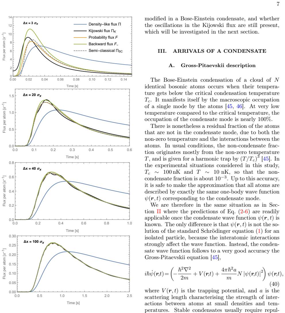
Arrivals on a vertical detector Let us now consider horizontal arrivals on the verti- cal detector, which are not directlty affected by grav- ity. The distributions of Eqs. (34-38) are illustrated in Fig. 4 for an isolated helium-4 atom initially held in a trap of frequencyωx = 2π×20Hz, for different detector positions∆x. Note that there is now only one s...
2000
-
[14]
(41), yielding |ψ0(r)|2 ≈ |ψTF(r)|2 ≡max 0, µ−V(r) 4πℏ2N a/m (47) where the chemical potential is found from Eq
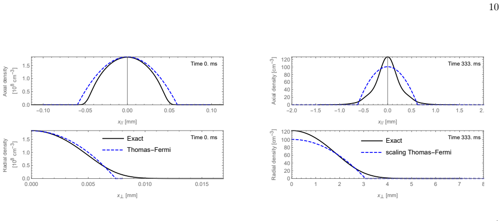
Thomas-Fermi approximation The initial density profile can be captured in the limit of largeN aby the Thomas-Fermi approxima- tion, which consists in neglecting the kinetic term in Eq. (41), yielding |ψ0(r)|2 ≈ |ψTF(r)|2 ≡max 0, µ−V(r) 4πℏ2N a/m (47) where the chemical potential is found from Eq. (25) and Eq. (42) to be [45], µ= 1 2 ℏ¯ω(15N a/¯σ)2/5 (48) ...
-
[15]
II exactly satisfies the scaling approximation with the scaling factorsλ i(t) = p 1 +ω 2 i t2 — see Eq
Scaling approximation The expansion dynamics can be captured to a great extent by assuming that the rescaled functionϕis time-independent, so that only the scaling factorsλi(t) account for the dynamics: ψ(r, t)≈ϕ ri λi(t) e i m 2ℏ P j r2 j ˙λj(t) λj(t) Q j λj(t)1/2 .(52) In that case, the integrated densities ni(ri, t)≡ Z drjdrk |ψ(r, t)|2 (53) satisfy th...
-
[16]
pancake” limit (ω∥ ≫ω ⊥), the symmetric case (ω∥ =ω ⊥), and the “cigar
Scaling Thomas-Fermi approximation The scaling Thomas-Fermi approximation corre- sponds to the conjonction of the two preceding ap- proximations, i.e. the initial state is assumed to be in the Thomas-Fermi limit Eq. (47) and the dynam- ics is assumed to follow the scaling approximation. In that case, the scaling factorsλi are found to obey the equations [...
-
[17]
Arrival-time distribution In the scaling Thomas-Fermi approximation, one can analytically calculate the first three arrival-time distributions Eq. (2-6) for arrivals along directionion a planar surfaceSperpendicular to it: Π(t) =α 1 λi(t) ni ri λi(t) ,0 (61) F(t) = ℏ mRTF i ri RTF i 1 λi(t)2 B(t)ni(ri, t)(62) F−(t) = ℏ mRTF i ri RTF i 1 λi(t)2 (B(t) +A(r ...
-
[18]
This results in a cigar-shaped Bose-Einstein condensate as an initial state
Setup To describe a typical experiment, we consider a con- densate of104 metastable helium-4 atoms (a= 7.5nm) held in a harmonic trap of cylindrical symmetry, with axial trapping frequencyω ∥ = 2π×25Hz and trans- verse frequencyω ⊥ = 2π×200Hz. This results in a cigar-shaped Bose-Einstein condensate as an initial state. The density cuts along the symmetry ...
-
[19]
In this con- figuration, the detector monitors the arrivals along a transverse direction of the condensate
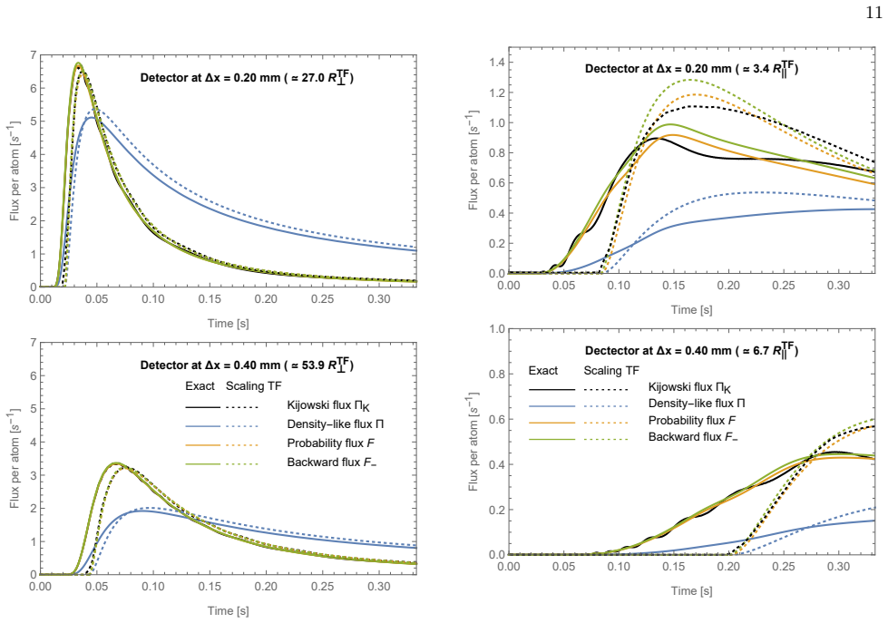
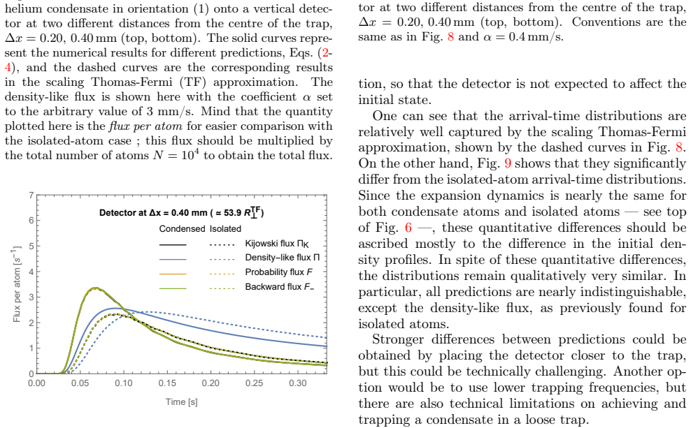
Vertical trap axis: transverse arrivals We first consider the orientation (1) of the conden- sate, for which the trap axis is vertical. In this con- figuration, the detector monitors the arrivals along a transverse direction of the condensate. The different predictions for the arrival-time distri- bution are shown in Fig. 8 for two distances of the detect...
-
[20]
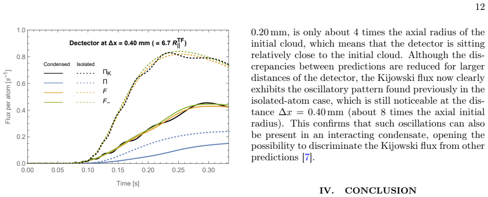
Horizontal trap axis: axial arrivals We now consider the orientation (2) of the initial cloud, for which the trap axis is horizontal and perpen- dicular to the vertical detector. In that configuration, 12 0.00 0.05 0.10 0.15 0.20 0.25 0.30 0.0 0.2 0.4 0.6 0.8 1.0 Time[s] Flux per atom[s -1] Dectector atΔx=0.40 mm(≃6.7R ||TF) Condensed Isolated ΠK Π F F- F...
-
[21]
M. H. Anderson, J. R. Ensher, M. R. Matthews, C. E. Wieman, and E. A. Cornell, Science269, 198 (1995)
1995
-
[22]
K. B. Davis, M. O. Mewes, M. R. Andrews, N. J. van Druten, D. S. Durfee, D. M. Kurn, and W. Ketterle, 13 Phys. Rev. Lett.75, 3969 (1995)
1995
-
[23]
Robert, O
A. Robert, O. Sirjean, A. Browaeys, J. Poupard, S. Nowak, D. Boiron, C. I. Westbrook, and A. Aspect, Science292, 461 (2001)
2001
-
[24]
Pauli, inPrinciples of Quantum Theory I, En- cyclopedia of Physics, Vol
W. Pauli, inPrinciples of Quantum Theory I, En- cyclopedia of Physics, Vol. 5/1, edited by S. Flügge (Springer, 1958) p. 60
1958
-
[25]
Paul, Annalen der Physik464, 252 (1962)
H. Paul, Annalen der Physik464, 252 (1962)
1962
-
[26]
Muga and C
J. Muga and C. Leavens, Physics Reports338, 353 (2000)
2000
-
[27]
Naidon, L
P. Naidon, L. Happ, and D. Boiron, unpublished (2025)
2025
-
[28]
Giovannetti, S
V. Giovannetti, S. Lloyd, and L. Maccone, Phys. Rev. D92, 045033 (2015)
2015
-
[29]
Maccone and K
L. Maccone and K. Sacha, Phys. Rev. Lett.124, 110402 (2020)
2020
-
[30]
S. Roncallo, K. Sacha, and L. Maccone, Quantum7, 968 (2023), arXiv:2205.02219v4
-
[31]
D. N. Page and W. K. Wootters, Phys. Rev. D27, 2885 (1983)
1983
-
[32]
Aharonov and T
Y. Aharonov and T. Kaufherr, Phys. Rev. D30, 368 (1984)
1984
-
[33]
Aharonov and D
Y. Aharonov and D. Bohm, Phys. Rev.122, 1649 (1961)
1961
-
[34]
Allcock, Annals of Physics53, 286 (1969)
G. Allcock, Annals of Physics53, 286 (1969)
1969
-
[35]
Kijowski, Reports on Mathematical Physics6, 361 (1974)
J. Kijowski, Reports on Mathematical Physics6, 361 (1974)
1974
-
[36]
N. Grot, C. Rovelli, and R. S. Tate, Phys. Rev. A54, 4676 (1996)
1996
-
[37]
Delgado and J
V. Delgado and J. G. Muga, Phys. Rev. A56, 3425 (1997)
1997
-
[38]
Anastopoulos and N
C. Anastopoulos and N. Savvidou, Journal of Mathe- matical Physics47, 122106 (2006)
2006
-
[39]
Allcock, Annals of Physics53, 253 (1969)
G. Allcock, Annals of Physics53, 253 (1969)
1969
-
[40]
Allcock, Annals of Physics53, 311 (1969)
G. Allcock, Annals of Physics53, 311 (1969)
1969
-
[41]
Werner, Journal of Mathematical Physics27, 793 (1986)
R. Werner, Journal of Mathematical Physics27, 793 (1986)
1986
-
[42]
Aharonov, J
Y. Aharonov, J. Oppenheim, S. Popescu, B. Reznik, and W. G. Unruh, Phys. Rev. A57, 4130 (1998)
1998
-
[43]
A. D. Baute, R. S. Mayato, J. P. Palao, J. G. Muga, and I. L. Egusquiza, Phys. Rev. A61, 022118 (2000)
2000
-
[44]
E. A. Galapon, F. Delgado, J. G. Muga, and I. n. Egusquiza, Phys. Rev. A72, 042107 (2005)
2005
-
[45]
Jurić and H
T. Jurić and H. Nikolić, Eur. Phys. J. Plus137, 631 (2022)
2022
-
[46]
Kijowski, Phys
J. Kijowski, Phys. Rev. A59, 897 (1999)
1999
-
[47]
Leavens, Physics Letters A303, 154 (2002)
C. Leavens, Physics Letters A303, 154 (2002)
2002
-
[48]
Egusquiza, J
I. Egusquiza, J. Muga, B. Navarro, and A. Ruschhaupt, Physics Letters A313, 498 (2003)
2003
-
[49]
Leavens, Physics Letters A345, 251 (2005)
C. Leavens, Physics Letters A345, 251 (2005)
2005
-
[50]
Madelung, Zeitschrift für Physik40, 322 (1927)
E. Madelung, Zeitschrift für Physik40, 322 (1927)
1927
-
[51]
W. R. McKinnon and C. R. Leavens, Phys. Rev. A51, 2748 (1995)
1995
-
[52]
C. R. Leavens, Phys. Rev. A58, 840 (1998)
1998
-
[53]
Bohm, Phys
D. Bohm, Phys. Rev.85, 166 (1952)
1952
-
[54]
Bohm, Phys
D. Bohm, Phys. Rev.85, 180 (1952)
1952
-
[55]
Fényes, Zeitschrift für Physik132, 81 (1952), [A probabilistic foundation and interpretation of quan- tum mechanics]
I. Fényes, Zeitschrift für Physik132, 81 (1952), [A probabilistic foundation and interpretation of quan- tum mechanics]
1952
-
[56]
Nelson, Phys
E. Nelson, Phys. Rev.150, 1079 (1966)
1966
-
[57]
Nelson,Quantum fluctuations, Vol
E. Nelson,Quantum fluctuations, Vol. 108 (Princeton University Press, 1985)
1985
-
[58]
Naidon, Phys
P. Naidon, Phys. Rev. A109, 063312 (2024)
2024
-
[59]
H.NittaandT.Kudo,Phys.Rev.A77,014102(2008)
2008
-
[60]
E. H. Kennard, Zeitschrift für Physik44, 326 (1927)
1927
-
[61]
Zimmermann, M
M. Zimmermann, M. A. Efremov, A. Roura, W. P. Schleich, S. A. DeSavage, J. P. Davis, A. Srinivasan, F. A. Narducci, S. A. Werner, and E. M. Rasel, Appl. Phys. B123(2017)
2017
-
[62]
Aveline, J
D. Aveline, J. Williams, and E. E. et al., Nature582, 193 (2020)
2020
-
[63]
W. Cavendish, S. Das, M. Nöth, and A. A. Raf- sanjani, arXiv preprint quant-ph/2409.00161 (2024), arXiv:2409.00161 [quant-ph]
- [64]
-
[65]
C. J. Pethick and H. Smith,Bose–Einstein Condensa- tion in Dilute Gases, 2nd ed. (Cambridge University Press, 2008)
2008
-
[66]
Castin,Condensats de Bose-Einstein(EDP Sci- ences, 2025)
Y. Castin,Condensats de Bose-Einstein(EDP Sci- ences, 2025)
2025
-
[67]
C. M. Dion and E. Cancès, Computer Physics Com- munications177, 787 (2007)
2007
-
[68]
A. S. Bradley, J. Clarke, T. W. Neely, and B. P. An- derson, Phys. Rev. A106, 053316 (2022)
2022
-
[69]
Castin and R
Y. Castin and R. Dum, Phys. Rev. Lett.77, 5315 (1996)
1996
discussion (0)
Sign in with ORCID, Apple, or X to comment. Anyone can read and Pith papers without signing in.