Pith. sign in

REVIEW 3 major objections 6 minor 2 cited by

No existing or planned 8 m-class instrument combines multi-object spectroscopy with R=80 000 resolution and 10 m/s radial-velocity stability; HRMOS is designed to fill that gap.

Reviewed by Pith at T0; open to challenge. T0 means a machine referee read the full paper against a public rubric. the ladder, T0–T4 →

HRMOS is proposed as a VLT instrument delivering R=80 000 multi-object spectroscopy with 10 m s^{-1} RV precision for 50-60 targets simultaneously, enabling large-sample high-fidelity studies of stars and gas.

T0 review reviewed 2026-07-11 challenge →

load-bearing objection Solid VLT 2030 white paper that correctly identifies a real capability gap and backs the science with concrete simulations; the RV budget is the main engineering risk, not a science-case failure. the 3 major comments →

arxiv 2607.04916 v1 pith:2UT3MZSV submitted 2026-07-06 astro-ph.IM astro-ph.GAastro-ph.SR

HRMOS: A High-Resolution Multi-Object Spectrograph for the VLT

Laura Magrini , Thomas Bensby , Sofia Randich , Andrea Bianco , Oscar Gonzalez , Emma Fernandez-Alvar , Sergio G. Sousa , Letizia Caito
show 169 more authors
Marco Riva Vardan Adibekyan Anish M. Amarsi Maria Teresa Belmonte Maria Benito Christian P. Clear Camilla Danielski Valentina D'Orazi Riano Giribaldi Camilla J. Hansen Vanessa Hill Robin D. Jeffries Georges Kordopatis Andrea Miglio Dinko Milakovic Germano Sacco Jose Schiappacasse-Ulloa Asa Skuladottir Rodolfo Smiljanic Maria Tsantaki Almudena Arcones Jose Maria Arroyo-Polonio Martina Baratella Beatriz Barbuy John R. Barnes Giuseppina Battaglia Holger Baumgardt Katia Biazzo Manuela Bischetti Angela Bragaglia Tobias Buck Sven Buder Sema Caliskan Gabriele Cescutti Andrew Collier Cameron Ryan Cooke Sergio Cristallo Francesco Damiani Arnas Drazdauskas Heitor Ernandes Antonio Frasca Mark Gieles Valeria Grisoni Moira Jardine Evan N. Kirby Jonas Klevas Andreas Korn Ioanna Koutsouridou Cis Lagae Nadege Lagarde Romain Lucchesi Francesca Lucertini Luca Malavolta Fabiola Marino Tadafumi Matsuno Thibault Merle Sapna Mishra Marta Molero Mario Montalto Michele Moresco Alessio Mucciarelli Domenico Nardiello Valerio Nascimbeni Brunella Nisini Joana Oliveira Elenia Pacetti Marco Palla Marco Pignatari Danae Polychroni Federico Rizzuti Donatella Romano Stefania Salvadori Luca Sbordone Emanuele Spitoni Matthew R. Standing Grazina Tautvaivsiene Yuan-Sen Ting Andrea Travascio Diego Turrini Sophie Van Eck Kim Venn Diego Vescovi C. Clare Worley Nick Wright Robert Yates Alice Zocchi Laura Affer Carlos Allende Paul Barklem Michele Bellazzini Serena Benatti Leda Berni Francesco Borsa Maurizio Busso Tiago Campante Roberta Carini Brad Carter Giada Casali Mario Damasso Elisa Delgado Mena Ignacio Del Moral Castro Silvano Desidera Maria Pia Di Mauro Ana Escorza Sergio Fonte Elena Franciosini Xiaoting Fu Paolo Giacobbe Terese Thidemann Hansen Henrik Hartman Keith Hawkins Neda Heidari Krzysztof Helminiak H. Jens Hoeijmakers Stavro Lambrov Ivanovski Pascale Jablonka Chiaki Kobayashi Arunas Kucinskas Carmela Lardo Sebastiano Ledda Alesandra Lehtmets Karin Lind Jo\~ao J.G. Lima Sara Lucatello Fatemeh Zahra Majidi Sarah Martell Anna McLeod Sergio Molinari Stephanie Monty Benjamin Montet Michael T. Murphy Henryka Netzel-I{\l}kiewicz Belinda Nicholson Patrick Palmeri Luca Pasquini Lorenzo Pino Romolo Politi Francesca Primas Pascal Quinet Monica Rainer Heleri Ramler Yassin Rany Khalil Martina Rossi Eugenio Schisano Federico Sestito Paolo Simonetti Arianna Vasini Silvia Vicente Carlos Viscasillas Vazquez Manuela Zocchi Michele Zusi Andrea Baruffolo Martin Black Anna Brucalassi Simone D'Auria Vincenzo De Caprio Michele Frangiamore Enrico Giro Robert J. Harris Alen Khanbekyan Enrique Joven Tom Louth Matteo Munari Graham J. Murray Luis Fernando Rodriguez Ramos Bernardo Salasnich William Taylor Andrea Tozzi Steven Watson
This is my paper
classification astro-ph.IM astro-ph.GAastro-ph.SR
keywords high-resolution spectroscopymulti-object spectrographVLT instrumentationradial velocitystellar abundancesnucleocosmochronologyexoplanets in clustersGalactic archaeology
verification ladder T0 review T1 audit T2 compute T3 formal T4 reserved

The pith

A machine-rendered reading of the paper's core claim, the machinery that carries it, and where it could break.

The reading

This white paper argues that astronomy needs an instrument that can observe dozens of stars at once at very high spectral resolution with metre-per-second radial-velocity stability, and that no current or planned facility on an 8-metre telescope does both. HRMOS is proposed for the VLT to deliver resolving power R=80 000, 50–60 simultaneous targets, optical coverage down to 385 nm, and 10 m/s (goal 5 m/s) radial-velocity precision. With those capabilities, large samples in crowded fields—open and globular clusters, the Galactic bulge, and nearby dwarf galaxies—can be measured for precise abundances, isotopic ratios, line profiles, and velocities. The paper claims this combination will settle open questions on the ages of the oldest stars, planet occurrence across environments, the origin of the heaviest elements, and the assembly of the Milky Way and its satellites. It presents the design heritage from FLAMES and MOONS, the technical architecture, and the science cases that set the top-level requirements.

Core claim

The central claim is that a single VLT instrument combining multiplex of 50–60 fibres, resolving power R=80 000, blue coverage to 385 nm, and residual radial-velocity precision of order 10 m/s will enable statistically large, high-fidelity spectroscopic studies in crowded fields that are infeasible with either pure multi-object survey spectrographs or single-object ultra-stable spectrographs alone.

What carries the argument

The baseline HRMOS instrument concept: a hybrid front-end fibre positioner with dual-zone atmospheric dispersion correction, double-scrambling fibre link with image slicers, three VPH-grating spectrograph arms under thermal/pressure control, and simultaneous laser-frequency-comb calibration, sized to meet an RV error budget of roughly 8 m/s total.

Load-bearing premise

That the hybrid positioner, double scrambling, stabilised spectrographs and simultaneous calibration will actually keep residual radial-velocity systematics at or below about 7 m/s under real Nasmyth operating conditions.

What would settle it

On-sky commissioning and stability campaigns that measure the delivered multi-fibre RV floor; if the residual systematic error substantially exceeds the 10 m/s requirement after calibration, the exoplanet-occurrence and precise-kinematics science cases fail as stated.

Watch this falsifier. Get emailed when new claim-graph text bears on it.

If this is right

  • Complete surveys of giant-planet occurrence become feasible in open and globular clusters and in bulge and dwarf-galaxy fields with well-known ages and metallicities.
  • Nucleocosmochronology ages from Th/Eu (and U) can be averaged over many members of the oldest globular clusters, giving a model-independent lower bound on the age of the Universe.
  • Full abundance patterns and Ba isotopic fractions for large samples of metal-poor stars and accreted populations can distinguish r-, s- and i-process sites and map hierarchical assembly of the Magellanic Clouds and Sagittarius.
  • High-precision light-element and isotopic work (C isotopes, S, Mg isotopes) in coeval cluster stars can calibrate mixing, diffusion and polluter models for multiple populations.
  • HRMOS becomes the natural high-resolution bridge between large surveys (4MOST, Gaia, PLATO) and ELT single-object instruments such as ANDES.

Where Pith is reading between the lines

These are editorial extensions of the paper, not claims the author makes directly.

  • If the dual-ADC hybrid architecture works as budgeted, it may become a template for other high-stability multi-object designs that need both crowded-field packing and full optical wavelength coverage.
  • Failure to meet the RV floor would still leave a powerful abundance and isotope machine; the white paper’s science portfolio is broader than the exoplanet case alone.
  • The explicit coupling of the instrument to laboratory atomic data and 3D non-LTE atmosphere grids implies that first-light science return depends as much on those community deliverables as on hardware.
  • A successful HRMOS would pressure future survey facilities to plan explicit high-resolution follow-up pathways rather than treating R~20 000 as the end point.
Share X Bluesky LinkedIn Reddit HN

Editorial analysis

A structured set of objections, weighed in public.

Desk editor's note, referee report, simulated authors' rebuttal, and a circularity audit.

Referee Report

3 major / 6 minor

Summary. This White Paper presents the scientific rationale and baseline instrument concept for HRMOS, a proposed VLT Nasmyth multi-object spectrograph combining R=80 000, 50–60 fibres, optical coverage down to ~385 nm, and a radial-velocity precision requirement of 10 m s^{-1} (goal 5 m s^{-1}). It argues that no existing or planned 8 m-class facility offers this combination, and that the design enables statistically significant high-fidelity abundance, isotope, line-profile and RV studies in crowded fields (open/globular clusters, bulge, nearby dwarfs). Science drivers span exoplanet occurrence across environments, nucleosynthesis (C isotopes, S, s/i/r-process and Ba isotopes), hierarchical assembly of MW satellites, nucleocosmochronology (Th/Eu), cluster physics, and ISM/CGM absorption. Technical heritage from FLAMES/MOONS, a dual-zone ADC hybrid positioner, double scrambling, three VPH arms and simultaneous LFC calibration is summarised, with an RV error budget claiming ~8.2 m s^{-1} total residual.

Significance. If the instrument is built and meets its TLRs, it would occupy a genuinely empty region of the MOS–resolution–stability parameter space and provide a natural bridge between 4MOST/Gaia/PLATO-class surveys and ELT/ANDES single-object work. The science cases are unusually well supported for a white paper: concrete RV detectability maps, HRMOS-like spectrum translators from ESPRESSO/HARPS, synthetic spectra for C isotopes, S I Multiplet 8, Ba isotopes, Th/Eu, Mg precision vs SNR, and binary recovery simulations give falsifiable performance targets. Explicit integration of laboratory atomic data and expanded 3D RHD/non-LTE modelling into the project plan is a strength. The document is therefore a credible community input to the VLT 2030 process rather than a pure advocacy brochure.

major comments (3)
  1. §1.3.8 and Table 1.2 (Eqs. 1.1–1.5): The residual systematic budget of ~6.7 m s^{-1} (total ~8.2 m s^{-1}) is load-bearing for the exoplanet occurrence-rate and precise-kinematics cases (Ch. 2, §6.6). The budget assumes double-scrambling gain ~10^4, ~30% LFC calibration residuals, and thermo-mechanical control at a few mK h^{-1}. Under real VLT Nasmyth thermal/pressure cycles, dual-zone ADC residuals, fibre stress and operational overheads these terms may exceed the allocation. The manuscript should add a short risk/mitigation subsection quantifying which science products survive if residual systematics are 15–20 m s^{-1} rather than ~7 m s^{-1}, and which require the goal 5 m s^{-1}.
  2. §1.3.3–1.3.4 (hybrid r–θ / pick-and-place dual-ADC architecture): The dual-zone solution (central common ADC for ≥10 arcsec separation; peripheral per-fibre ADCs for ≥30 arcsec) is central to crowded-field science (GC cores, bulge). Technology readiness is asserted by analogy to ESPRESSO/MOONS/KMOS, but no quantitative residual-dispersion or coupling-efficiency budget across the 385–677 nm range is given for the two zones. A table or figure of expected ADC residual vs airmass and zone would make the 10-arcsec inner-field claim more defensible.
  3. Executive summary and Ch. 8–9: Success of abundance/isotope science is conditioned on laboratory atomic data and expanded 3D RHD + multi-element non-LTE grids being available before first light. This is stated as a proactive project component, but no schedule, resource envelope or success metrics are given. Because several key diagnostics (Th, U, Ba isotopes, weak S I, heavy n-capture lines) are systematics-limited rather than photon-noise-limited, the White Paper should identify which science cases remain robust if only partial atomic/3D grids are delivered by first light.
minor comments (6)
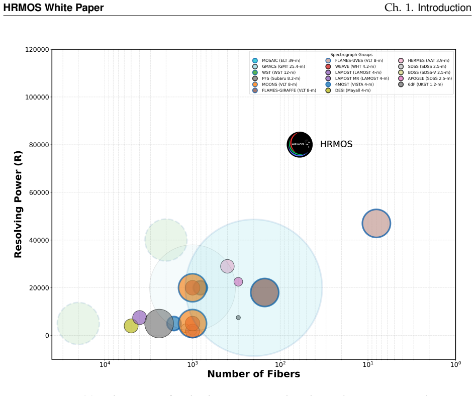
  1. Fig. 1.6 and 1.7: Symbol sizes and colour coding for multiplex and telescope aperture are useful, but the caption of Fig. 1.7 should state explicitly which instruments are integral-field vs multi-object vs single-object to avoid misreading the crowded legend.
  2. Table 1.2: Units are listed as cms^{-1} while the text discusses m s^{-1}; the conversion is clear but a consistent unit choice (or dual labelling) would reduce reader friction.
  3. §2.4.2: The HRMOS-like spectrum translator is a valuable tool; stating whether the code will be public (and under what licence) would strengthen reproducibility claims.
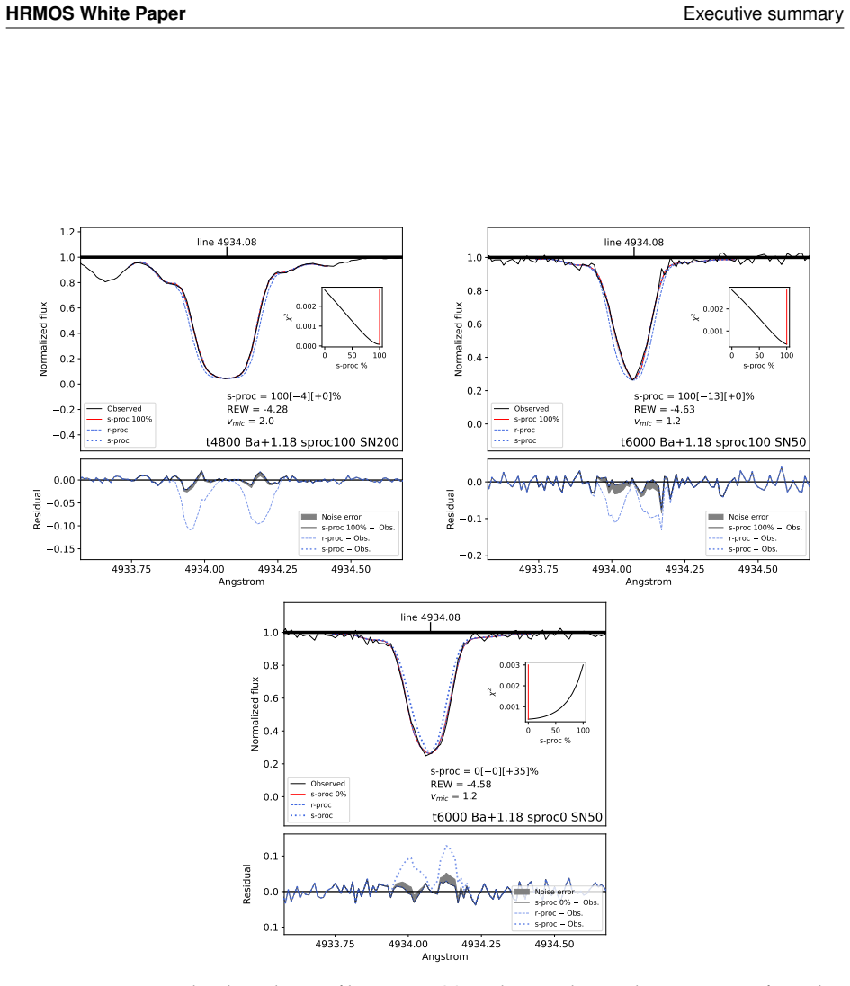
  4. §3.4.3 / Fig. 3.4: Ba-isotope residual panels are informative; adding the corresponding UVES-like residual amplitude in the same figure (already discussed in text) would make the factor-of-two gain immediately visual.
  5. Chapter 11 observational strategies are concrete; a single summary table of nights-per-science-case (exoplanets, GCs, LMC/SMC/Sgr, bulge) would help readers and time-allocation committees.
  6. Acronym list is comprehensive; ensure first use of every acronym in the main text is expanded (a few late-chapter first uses appear only as acronyms).

Circularity Check

0 steps flagged

No circular derivation: instrument white paper with requirements flowing from science drivers and engineering estimates, not self-referential predictions.

full rationale

HRMOS is a design-and-science-case White Paper, not a first-principles derivation of a physical result. Top-level requirements (R=80 000, RV precision 10 m s^{-1} goal 5 m s^{-1}, 50–60 fibres, coverage to 385 nm; Table 1.1) are stated as design targets motivated by the science chapters; the instrument concept and RV error budget (Section 1.3.8, Table 1.2, Eqs. 1.1–1.5) are engineering estimates under stated assumptions (double scrambling gain ~10^4, LFC calibration residual factor ~3, N_lines ~800, etc.), not parameters fitted to data and then re-presented as independent predictions. Detectability simulations (Ch. 2), abundance/isotope feasibility spectra (Ch. 3–5), and target strategies (Ch. 11) are forward calculations given those design parameters. Self-citations (Magrini et al. 2023 first White Paper, Brucalassi et al. 2022, Riva et al. 2026, workshop presentations) document prior concept development and community process; none supply a uniqueness theorem or load-bearing premise that forces the performance claims. Uniqueness of the R–multiplex niche (Figs. 1.6–1.7) is an external landscape comparison, not a self-referential renaming. No self-definitional loop, fitted-input-as-prediction, or ansatz smuggled via citation reduces a central claim to its inputs by construction. Score 0 is the proportionate finding.

Axiom & Free-Parameter Ledger

4 free parameters · 5 axioms · 0 invented entities

As a design proposal the paper rests on engineering and community-science assumptions rather than free parameters fitted to data. The free parameters are the top-level requirements chosen by the consortium; the axioms are standard instrumental and astrophysical premises; no new physical entities are invented.

free parameters (4)
  • Resolving power R = 80000
    Baseline set to 80 000 by science-case trade-off; not derived from first principles.
  • RV precision requirement = 10 m s^{-1} (goal 5)
    Set to 10 m s^{-1} (goal 5) to enable hot-Jupiter detection and kinematics; drives the entire error budget.
  • Multiplex (number of fibres) = 50-60
    50 (goal 60) chosen as compromise between packing density, ADC packaging and spectrograph real-estate.
  • Spectral windows (central wavelengths) = three windows ~385-677 nm
    402, 501, 650 nm selected to cover key diagnostic lines; total coverage ~130 nm.
axioms (5)
  • domain assumption No existing or funded 8 m-class instrument combines R≳50 000 with multiplex ≳20 and RV stability ≲10 m s^{-1}.
    Stated in §1.2 and Figs. 1.6-1.7; underpins the entire 'gap' claim.
  • domain assumption Double scrambling yields a gain factor ~10^4, reducing guiding-induced RV systematics to sub-cm s^{-1}.
    §1.3.5 and error budget; standard but not re-demonstrated here.
  • domain assumption Simultaneous LFC calibration reduces residual systematics by a factor ~3 (30 % residuals).
    Table 1.2; conservative estimate drawn from HARPS/ESPRESSO experience.
  • domain assumption Science questions listed (nucleocosmochronology ages, cluster exoplanet occurrence, r-process sites, hierarchical assembly of LMC/SMC/Sgr) will remain open and high-priority in the 2030s.
    Executive summary and chapter introductions; necessary for strategic justification.
  • ad hoc to paper Adequate laboratory atomic data and expanded 3D RHD + multi-element non-LTE grids will be available by first light.
    Chapters 8-9 explicitly integrate these as deployment requirements; without them abundance precision claims degrade.

reviewed 2026-07-11 · how reviews work

0 comments
Cite this review

Pith. "Pith review of HRMOS: A High-Resolution Multi-Object Spectrograph for the VLT." pith.science (2026). https://pith.science/paper/2UT3MZSV

@misc{pith2026260704916,
  author       = {Pith},
  title        = {Pith review of: HRMOS: A High-Resolution Multi-Object Spectrograph for the VLT},
  year         = {2026},
  howpublished = {\url{https://pith.science/paper/2UT3MZSV}},
  note         = {Machine review of arXiv:2607.04916}
}
Share X Bluesky LinkedIn Reddit HN
read the original abstract

This White Paper presents the scientific rationale and instrument concept for HRMOS (High-Resolution Multi-Object Spectrograph), a next-generation instrument proposed for the ESO Very Large Telescope within the VLT 2030 roadmap. Current and planned facilities offer either multi-object spectroscopy or ultra-high spectral resolution, but not both. HRMOS fills this gap by combining very high spectral resolution, multi-object capability, and radial-velocity stability, enabling transformative studies in Galactic and extragalactic astrophysics. The baseline design provides a resolving power of R = 80000, radial-velocity precision of 10 m s-1 (goal: 5 m s-1), simultaneous observations of 50-60 targets, and broad optical coverage down to 385 nm. These capabilities enable precise measurements of elemental abundances, isotopic ratios, line profiles, and radial velocities for large stellar samples, including crowded fields, star clusters, the Galactic bulge, and nearby dwarf galaxies. HRMOS will address key questions on the age of the oldest stellar populations through nucleocosmochronology, the formation and survival of planetary systems, the assembly history of the Milky Way and satellites, the origin of the heaviest elements, stellar evolution, and the chemical and dynamical properties of the interstellar and circumgalactic medium. It will bridge large spectroscopic surveys and the next generation of extremely large telescopes, with strong synergies with 4MOST, Gaia, TESS, PLATO, the proposed Haydn mission, and future ELT instruments. Building on VLT/FLAMES heritage, HRMOS represents a strategic investment for European astronomy in the 2030s.

Figures

Figures reproduced from arXiv: 2607.04916 by Alen Khanbekyan, Alesandra Lehtmets, Alessio Mucciarelli, Alice Zocchi, Almudena Arcones, Ana Escorza, Andrea Baruffolo, Andrea Bianco, Andrea Miglio, Andreas Korn, Andrea Tozzi, Andrea Travascio, Andrew Collier Cameron, Angela Bragaglia, Anish M. Amarsi, Anna Brucalassi, Anna McLeod, Antonio Frasca, Arianna Vasini, Arnas Drazdauskas, Arunas Kucinskas, Asa Skuladottir, Beatriz Barbuy, Belinda Nicholson, Benjamin Montet, Bernardo Salasnich, Brad Carter, Brunella Nisini, Camilla Danielski, Camilla J. Hansen, Carlos Allende, Carlos Viscasillas Vazquez, Carmela Lardo, C. Clare Worley, Chiaki Kobayashi, Christian P. Clear, Cis Lagae, Danae Polychroni, Diego Turrini, Diego Vescovi, Dinko Milakovic, Domenico Nardiello, Donatella Romano, Elena Franciosini, Elenia Pacetti, Elisa Delgado Mena, Emanuele Spitoni, Emma Fernandez-Alvar, Enrico Giro, Enrique Joven, Eugenio Schisano, Evan N. Kirby, Fabiola Marino, Fatemeh Zahra Majidi, Federico Rizzuti, Federico Sestito, Francesca Lucertini, Francesca Primas, Francesco Borsa, Francesco Damiani, Gabriele Cescutti, Georges Kordopatis, Germano Sacco, Giada Casali, Giuseppina Battaglia, Graham J. Murray, Grazina Tautvaivsiene, Heitor Ernandes, Heleri Ramler, Henrik Hartman, Henryka Netzel-I{\l}kiewicz, H. Jens Hoeijmakers, Holger Baumgardt, Ignacio del Moral Castro, Ioanna Koutsouridou, Joana Oliveira, Jo\~ao J.G. Lima, John R. Barnes, Jonas Klevas, Jose Maria Arroyo-Polonio, Jose Schiappacasse-Ulloa, Karin Lind, Katia Biazzo, Keith Hawkins, Kim Venn, Krzysztof Helminiak, Laura Affer, Laura Magrini, Leda Berni, Letizia Caito, Lorenzo Pino, Luca Malavolta, Luca Pasquini, Luca Sbordone, Luis Fernando Rodriguez Ramos, Manuela Bischetti, Manuela Zocchi, Marco Palla, Marco Pignatari, Marco Riva, Maria Benito, Maria Pia Di Mauro, Maria Teresa Belmonte, Maria Tsantaki, Mario Damasso, Mario Montalto, Mark Gieles, Marta Molero, Martina Baratella, Martina Rossi, Martin Black, Matteo Munari, Matthew R. Standing, Maurizio Busso, Michael T. Murphy, Michele Bellazzini, Michele Frangiamore, Michele Moresco, Michele Zusi, Moira Jardine, Monica Rainer, Nadege Lagarde, Neda Heidari, Nick Wright, Oscar Gonzalez, Paolo Giacobbe, Paolo Simonetti, Pascale Jablonka, Pascal Quinet, Patrick Palmeri, Paul Barklem, Riano Giribaldi, Roberta Carini, Robert J. Harris, Robert Yates, Robin D. Jeffries, Rodolfo Smiljanic, Romain Lucchesi, Romolo Politi, Ryan Cooke, Sapna Mishra, Sarah Martell, Sara Lucatello, Sebastiano Ledda, Sema Caliskan, Serena Benatti, Sergio Cristallo, Sergio Fonte, Sergio G. Sousa, Sergio Molinari, Silvano Desidera, Silvia Vicente, Simone D'Auria, Sofia Randich, Sophie Van Eck, Stavro Lambrov Ivanovski, Stefania Salvadori, Stephanie Monty, Steven Watson, Sven Buder, Tadafumi Matsuno, Terese Thidemann Hansen, Thibault Merle, Thomas Bensby, Tiago Campante, Tobias Buck, Tom Louth, Valentina D'Orazi, Valeria Grisoni, Valerio Nascimbeni, Vanessa Hill, Vardan Adibekyan, Vincenzo de Caprio, William Taylor, Xiaoting Fu, Yassin Rany Khalil, Yuan-Sen Ting.

Figure 1.1
Figure 1.1. Figure 1.1: SNR per resolution element for F4V-, G2V, and K4V-type stars (left upper panel, right upper left and bottom panels, respectively) as a function of G magnitudes (Vega system) for 1 hr of exposure time (airmass 1, dark sky condition, seeing=0.8”). Section 1.3.7). The radial-velocity error budget for HRMOS is designed to meet a precision requirement of 10 m s−1 . According to technical simulations, the curr… view at source ↗
Figure 1.2
Figure 1.2. Figure 1.2: High-level block diagram of the HRMOS instrument, comprising the Front End, Fibre Link, Spectrographs, and Calibration Unit [PITH_FULL_IMAGE:figures/full_fig_p014_1_2.png] view at source ↗
Figure 1.3
Figure 1.3. Figure 1.3: Left: The r–θ positioner concept (derived from MOONS and KMOS designs) combines a rotation axis with a linkage mechanism enabling radial extension. Right: The novel pick-and-place concept with integrated miniaturised ADCs. reconfiguration and high fibre packing density; however, it would require a single, traditional telescope level ADC placed upstream of all fibres. This would likely require refractive … view at source ↗
Figure 1.4
Figure 1.4. Figure 1.4: Optical layout of the pick-and-place ADC sub-module for the peripheral zone (left: full collimator–ADC–camera train; right: pupil-concentric focal-plane arrangement within the Nasmyth rotator envelope). This hybrid solution represents the best compromise between two extremes: a single large ADC and a fully distributed system with one ADC per fibre. impractical at the scale of the central field. The techn… view at source ↗
Figure 1.5
Figure 1.5. Figure 1.5: Left: Block diagram of the HRMOS spectrographs. Right: Optical ray-trace layout of one HRMOS spectrograph arm, showing the pseudo-slit, collimator, VPH grating, and camera–detector assembly. The overall footprint is approximately 3.2 × 2.0 m Key design parameters. The main numerical parameters of each spectrograph arm are listed below. • Resolving power: R = 80 000 • Number of slices per science object: … view at source ↗
Figure 1.6
Figure 1.6. Figure 1.6: HRMOS in the context of multi-object spectrographs. The resolving power R is shown as a function of the number of fibres, with the symbol sizes proportional to the collecting area of the corresponding telescope. HRMOS is represented by its logo, positioned at R ≈ 80,000 and a multiplex of 60 fibres (within the range 50–60). Future instruments are represented with transparent circles; proposed facilities … view at source ↗
Figure 1.7
Figure 1.7. Figure 1.7: Positioning of HRMOS within the landscape of current and forthcoming ESO spectroscopic instrumentation in the optical and near-infrared ranges for VLT. The multi-object facilities are colour coded by the number of fibres or slits, which is reported in the legend. Single object and integrated field spectrographs are shown with different colours, as indicated in the top-right legend. The y axes is represen… view at source ↗
Figure 2.1
Figure 2.1. Figure 2.1: The planetary mass versus the orbital period for currently known exoplanets discovered either through the transit (orange) or Doppler techniques (blue) (NASA Exoplanet Archive, May 2026). Even after their growth and accretion phases are finished, exoplanets still experience physical changes. Gas giants should cool and contract over billions of years (e.g. Fortney et al. 2007). Those that migrate close to… view at source ↗
Figure 2.2
Figure 2.2. Figure 2.2: Simulations illustrating the regions where exoplanets become detectable with a 0.1 % false alarm probability. The four simulations are labelled with the mass of star considered and the level of starspot activity assumed. In each panel, regions are shown corresponding to instrumental velocity noise of 10 m s−1 and 30 m s−1 respectively. these conditions. An instrumental stability of 10 m s−1 allows detect… view at source ↗
Figure 2.3
Figure 2.3. Figure 2.3: Comparison between original ESPRESSO spectra (an observation from Tau Ceti) and HRMOS-like simulated spectra across different wavelength regions. The panels illustrate: B-band (top left), G-band (top right), R-band (bottom left), along with a zoomed-in view of the Sodium (Na) H line region (bottom right). Flux values are shown as a function of wavelength (in Å), highlighting the resolution degradation an… view at source ↗
Figure 2.4
Figure 2.4. Figure 2.4: Comparison between the uncertainties obtained in the analysis of the original ESPRESSO spectra of Tau Ceti (black dots) and HRMOS-like simulated spectra at SNR = 50 (yellow dots) and SNR = 100 (blue dots). The panel shows the resulting RV uncertainties: STD RV is the standard deviation of the RVs for each observation, while <eRV> is the average of the uncertainties of RVs for each observation. Note that … view at source ↗
Figure 2.5
Figure 2.5. Figure 2.5: Left: False Alarm Probability of detecting a planet around a single star with age of 120 Myr and no planetary companions, based on 30 observations simulated using a real ESPRESSO dataset. The blue and orange lines represent an analytical approximation to the 0.1% FAP from 30 and 50 observations, respectively. Right: Same as in the left plot, using as a baseline ESPRESSO observations of a 600 Myr star. Th… view at source ↗
Figure 2.6
Figure 2.6. Figure 2.6: Predicted environmental dependence of the giant planet formation efficiency. Top: normalised mass distributions of giant planets with mass greater than 0.3 MJ and orbiting at periods comprised between 1 and 10 days from the planetary population synthesis simulations performed for the three representative clusters NGC 2243, M67 and Rupercht 134 considering a 0.05 M⊙ solar nebula-like disc (see main text f… view at source ↗
Figure 2.7
Figure 2.7. Figure 2.7: Detection efficiency (with a 0.1,% false alarm probability) for exoplanets orbiting a 2 M⊙ giant star. The proposed 30 observations are distributed over a 5-year period as described in the text. Simulations assuming instrumental velocity precisions of 10 m s−1 or 30 m s−1 are shown. and dropping further to ≲1% in the metal-poor cluster ([Fe/H] ∼ −0.5), where the reduced solid content strongly inhibits ef… view at source ↗
Figure 2.8
Figure 2.8. Figure 2.8: Hexbin plot of the kima posterior samples obtained from runs on simulated datasets for EBLM J0310-31, with Np fixed to 1. The green curve shows the 3σ sensitivity limit calculated on posterior samples obtained from a kima run on 30 simulated HRMOS observations, while the blue curve shows the corresponding limit computed from the plotted posterior samples obtained from a run on 40 simulated HRMOS observat… view at source ↗
Figure 3.1
Figure 3.1. Figure 3.1: Spectral lines of neutron-capture elements that can be detected in the blue range of HRMOS at two resolving powers, R = 40k (top) and R = 80k (bottom). The simulations concerns a no-r-process enhanced red giant of [Fe/H] = −0.5. The size of the points indicate the purity with which the line can be measured and colour is related to the minimum signal-to-noise ratio needed (per pixel). It is clear that at … view at source ↗
Figure 3.2
Figure 3.2. Figure 3.2: Same as [PITH_FULL_IMAGE:figures/full_fig_p051_3_2.png] view at source ↗
Figure 3.3
Figure 3.3. Figure 3.3: Theoretical predictions of the evolution of the Ba isotopes in the Galactic halo: [Ba/Fe] versus [Fe/H] with the fraction of odd Ba isotopes in colour scale, highlighting the contribution from s-process (in red) or r-process (in blue). Model obtained with the GEMS code (Rizzuti et al. 2025). levels to the solar-system abundance. The three neutron-capture processes (s-, i-, and r-process) are expected to … view at source ↗
Figure 3.4
Figure 3.4. Figure 3.4: Fits to simulated Ba ii line profiles at HRMOS resolution. The simulations were performed as described for [Fe/H] = −1.5 dex. The effective temperature, A(Ba), s-process fraction, and SNR adopted in each case are reported in the lower-right corner of the panels, and the layout follows [PITH_FULL_IMAGE:figures/full_fig_p054_3_4.png] view at source ↗
Figure 3.5
Figure 3.5. Figure 3.5: Nucleosynthetic signature of the three neutron capture processes for [Fe/H] = −1.2 (top) and −2.2 (bottom). Neutron-capture elements To understand the precision of measurements of neutron-capture elements, additional simulations were performed for stars in six evolutionary stages. Three dwarfs in the main sequence with (Teff, log g) = (5800 K, 3.7), (6400 K, 4.1), and (6000 K, 4.5). And three red giants … view at source ↗
Figure 3.6
Figure 3.6. Figure 3.6: Simulated spectra of metal-rich dwarfs in regions containing 12CH and 13CH lines. −1.5, and −2.0 with [α/Fe] = 0.4 [PITH_FULL_IMAGE:figures/full_fig_p057_3_6.png] view at source ↗
Figure 3.7
Figure 3.7. Figure 3.7: Simulated S I 675.7 nm line in giant stars. Synthetic broadened spectra (black) and spectra with SNR = 100 (blue) are compared in the different cases. 56 [PITH_FULL_IMAGE:figures/full_fig_p058_3_7.png] view at source ↗
Figure 4.1
Figure 4.1. Figure 4.1: Predicted average number of mergers as a function of the stellar mass of the merging galaxy for the LMC (top), SMC (middle) and Sagittarius (bottom) galaxies. Left: CDM predictions for combinations of two galaxy occupation models (high and low threshold) and two SMHM relations (see Deason et al. 2022 for model details). Right: Predictions for the high and low threshold galaxy occupation models combined w… view at source ↗
Figure 4.2
Figure 4.2. Figure 4.2: Predicted [Zn/Fe] abundances for stars with > 50% PISN enrichment is shown with red color bar, in the Milky Way halo. Other predicted stars are shown in grey, and black symbols are measured abundances corrected for NLTE effects. Adopted from Koutsouridou et al. (2025). Clouds are most likely on their first infall (e.g. Besla et al. 2010), while Sagittarius shows clear evidence of tidal stripping (Ibata e… view at source ↗
Figure 4.3
Figure 4.3. Figure 4.3: The number of detected binaries with period, P, during simulated 5-year mock observations with 5 epochs for a typical dSph galaxy (Sculptor). Black lines show the assumed underlying distributions while coloured lines show different assumption of the radial velocity precision, σ◦ = 0.02 (red), 0.1 (green), 0.5 (blue) and 1 km s−1 (cyan). Credit: A. Sollima. characteristics (distribution of periods, mass-r… view at source ↗
Figure 4.4
Figure 4.4. Figure 4.4: Precision of Mg measurements as a function of SNR, assuming a typical evolved giant with log g = 1.5, and [Mg/Fe] = 0.0, measured from the two redder lines of the Mg i triplet at ∼518 nm. Strong wings of the lines at higher [Fe/H] result in less precision. tracer of the rapid neutron-capture process (from ccSN and NSM). The degree of blending with other lines in the 4MOST spectra adds greatly to the unce… view at source ↗
Figure 4.5
Figure 4.5. Figure 4.5: Synthetic spectra (black) for a typical star representative of our samples (Teff = 4500 K, log g = 1.0, [Fe/H] = −0.5) around the Al i 396.1 nm line (left), and the Eu ii 420.5 nm line (right) with HRMOS resolution (R=80,000) at the top, compared to 4MOST resolution (R=20,000) at the bottom. Red lines show the synthetic spectra without Al (left) or Eu (right) present. brighter stars for shorter exposure … view at source ↗
Figure 4.6
Figure 4.6. Figure 4.6: The three large and nearby Milky Way satellite galaxies, RGB members with G ≤ 16.5. Left: Spatial distribution of stars, colour coded by the number of stars per FoV (green circle, d = 25′ ). Right: Histogram of all stars with G ≤ 16.5 (blue) and those located in regions with densities ≥ 50 stars/FoV (orange). 67 [PITH_FULL_IMAGE:figures/full_fig_p069_4_6.png] view at source ↗
Figure 5.1
Figure 5.1. Figure 5.1: Simulated spectra in the region of the Th line (indicated with a vertical dotted line) at different resolution, as indicated in the legend. intrinsically stronger in the latter. We note that continuum normalisation can be challenging in metal-rich giants; however, this does not affect our science case, which is focused on metal-poor stars. We further investigate the abundance precision that can be achiev… view at source ↗
Figure 5.2
Figure 5.2. Figure 5.2: Target sky-density (in Galactic coordinates) for stars with different mass ranges (different rows) and metallicities (columns). Pixels are one square degree. A cut on the error in parallax, RUWE value and G magnitude G=15 has been applied (see Sect. 5.6). 76 [PITH_FULL_IMAGE:figures/full_fig_p078_5_2.png] view at source ↗
Figure 6.1
Figure 6.1. Figure 6.1: A normalised cumulative histogram of v sin i for solar-type stars (4000 < Teff/K < 6500) in clusters with ages from 5 − 300,Myr (data from the Gaia-ESO Survey, Randich et al. 2022). The vertical line marks the threshold where the rotation profile can be resolved into 10 elements at R = 80K. Approximately 20 − 40% of stars are viable targets for Doppler imaging in clusters of age 5 − 300 Myr. Lower-resolu… view at source ↗
Figure 6.2
Figure 6.2. Figure 6.2: Age–mass diagram of star clusters. Plus signs: open clusters in the MW; circles: MW GCs; squares: Magellanic Clouds and Fornax GCs. Red: multiple populations; light blue: absent; white: unclassified (figure from Bragaglia et al. 2017). tags. Combined with high-precision radial velocities, this will allow us to trace cluster dynamical evolution and test whether 1P stars were preferentially lost over time.… view at source ↗
Figure 6.3
Figure 6.3. Figure 6.3: HST chromosome maps using F275W, F336W, F438W, and F814W bands (Milone et al. 2017). The pseudo-colour index ∆CF275W, F336W, F438W = ∆[(F275W − F336W) − (F336W − F438W)] is plotted against ∆F275W − F814W. Left: NGC 3201 (Type I, classical 1P–2P dichotomy). Right: NGC 5286 (Type II) showing an additional subpopulation enriched in CNO and Fe (red triangles). Arrows indicate effects of specific abundance ch… view at source ↗
Figure 6.4
Figure 6.4. Figure 6.4: Expectations of HRMOS spectra around the MgH region tracing the three different Mg isotopes. Shown are spectra taken with the Veloce spectrograph at R = 80 000 of the metal-poor G dwarf Tau Cet (top), the K dwarf HIP 12114 (middle), and a red clump star (HIP48455, bottom) with solar metallicity. Tuc, Thygesen et al. (2016) found no variation in isotopic ratios. More recently, McKenzie et al. (2024) analy… view at source ↗
Figure 6.5
Figure 6.5. Figure 6.5 [PITH_FULL_IMAGE:figures/full_fig_p088_6_5.png] view at source ↗
Figure 6.6
Figure 6.6. Figure 6.6: Simulated Li I 670.8 nm doublet in giants at varying Li abundances (rows) and stellar parameters, assuming [Fe/H] = −0.5, [α/Fe] = 0.0, and SNR = 50. Black line, pure 7Li, blue line 6Li/7Li = 0.08. enabled by the high resolution of HRMOS. Although Li-rich giants are found in both field and cluster environments, globular clusters are particularly well suited for demographic studies due to their coeval, de… view at source ↗
Figure 6.7
Figure 6.7. Figure 6.7: Same as in [PITH_FULL_IMAGE:figures/full_fig_p092_6_7.png] view at source ↗
Figure 6.8
Figure 6.8. Figure 6.8: A simulated observation of the GC M4 with HRMOS. Top-right: the distribution of the observed stars. Top-left: the variation of the velocity dispersion σRV with the distance from the GC centre. Bottom￾left: the observed binary fraction as a function of the distance of the GC, assuming a binary fraction fbin = fbin(0)(R/RHM) 0.25, with fbin(0)= 0.1 (blue dots), 0.2 (orange dots), 0.3 (green dots). Bottom-r… view at source ↗
Figure 7.1
Figure 7.1. Figure 7.1: Three types of absorption systems that could be studied with HRMOS observations of extragalactic sources like quasars and AGN (see text for details). This image was created using generative large-language model Gemini 3, using the description of absorption systems as prompt. of AGN feedback. HRMOS observations, at a spectral resolution corresponding to 3–5 km s−1 , will enable the disentangling of these … view at source ↗
Figure 7.2
Figure 7.2. Figure 7.2: HRMOS can be used to study extragalactic gas in absorption towards quasars and other AGN. Based on known luminosity functions, a typical VLT field of view contains on average ∼ 8 AGN, including approximately one quasar. The figure illustrates a representative fibre allocation strategy. tools provide measurements of line widths, column densities, and redshifts of absorption systems, which can be used to c… view at source ↗
Figure 8.1
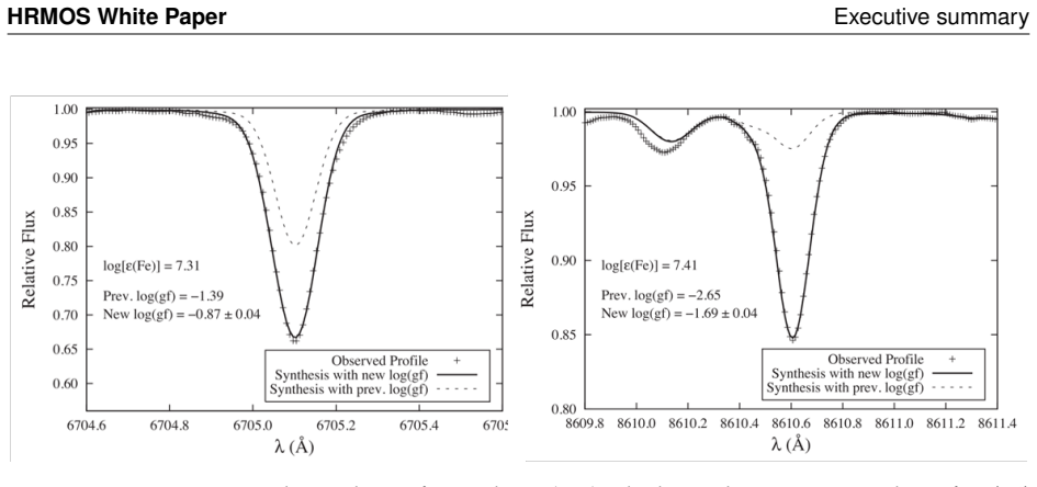
Figure 8.1. Figure 8.1: Improvement in the synthesis of neutral iron (Fe I) solar lines when using new values of log(gf) measured by Ruffoni et al. (2014) with a high-resolution Fourier transform spectrometer. The dotted lines show the synthesis using the previous best values. The importance of accurate laboratory transition probabilities is illustrated in [PITH_FULL_IMAGE:figures/full_fig_p105_8_1.png] view at source ↗
Figure 8.2
Figure 8.2. Figure 8.2: Synthetic spectra of Sm ii λ5069 showing the impact of both hyperfine and isotope structure on line profile (Lundqvist, M. et al. 2007). The dotted profile includes both HFS and IS, the dashed profile is IS only and the dot-dashed profile is without either HFS or IS. The difference between the lines with structure and without is ∼0.1 dex. structure in complex ions. The Co ii line at 261.51 nm is shown wi… view at source ↗
Figure 8.3
Figure 8.3. Figure 8.3: Observed (black) and fitted (red dashed) line profile of the Co ii 261.51 nm transition from Ding & Pickering (2020). The relative intensities of the individual HFS components are given by red lines. The transition diagram detailing individual hyperfine transitions is shown at the top of the figure. ionised (iv ) atoms (Heise et al. 1994). A third way of getting emission spectra, in this case from neutra… view at source ↗
Figure 8.4
Figure 8.4. Figure 8.4: Year of last large-scale energy level analysis of low-ionisation iron group elements. NIST Atomic Spectral Database (ASD, Kramida et al. (2024)) contains 40 lines in the HRMOS spectral region, only 12 of which include log(gf) values. Of these, only the two resonant lines (Srii 407.77 and 421.55 nm) have accurate log(gf) values (0.004 dex). The remaining ten lines, one of which (Srii 416.18 nm) is of inte… view at source ↗
Figure 9.1
Figure 9.1. Figure 9.1: Example of the temperature structure of a 3D box-in-a-star Stagger-model for the Sun. The colour is capped at 13000 K to improve the visual clarity of the surface inhomogeneities. Based on data presented in Rodríguez Díaz et al. (2024). Full movie available at https://warwick.ac.uk/fac/sci/physics/research/ astro/people/cislagae. The most commonly used grids are the Stagger-grid (Magic et al. 2013; Rodrí… view at source ↗
Figure 9.2
Figure 9.2. Figure 9.2: The Stagger-grid of 3D model atmospheres. Existing models are circles colour-coded by metallicity, missing models are made transparent. Overplotted are MIST stellar evolutionary tracks (Dotter 2016; Choi et al. 2016; Paxton et al. 2011, 2013, 2015) for two metallicities, [Fe/H] = 0, −2, and four stellar masses: 0.7 − 1.0 M⊙ in steps of 0.1 M⊙. Priority models for an expanded grid are solid squares. Adapt… view at source ↗
Figure 9.3
Figure 9.3. Figure 9.3: Impact of the model atom on spectral line strengths and thus on the [X/Fe] versus [Fe/H] plane (e.g. Chapters 4 and 3). Top: synthesis of the Cu I 510 nm line for a typical metal-poor red giant branch star in LTE, and in non-LTE with different prescriptions for the inelastic hydrogen collisions (left and right). Logarithmic reduced equivalent widths indicated in parentheses. Gaussian broadening correspon… view at source ↗
Figure 9.4
Figure 9.4. Figure 9.4: Solar Hα line profile fit. The observational spectrum (black line) has a resolving power R = 86 000, taken from the MELCHIORS public database (Royer et al. 2024) normalised as in Giribaldi et al. (2019). Vertical shaded regions indicate the portions of the spectrum used for fitting. The best-fit 3D non-LTE synthetic profile is shown as a solid red line, with the corresponding temperature labelled in the … view at source ↗
Figure 11.1
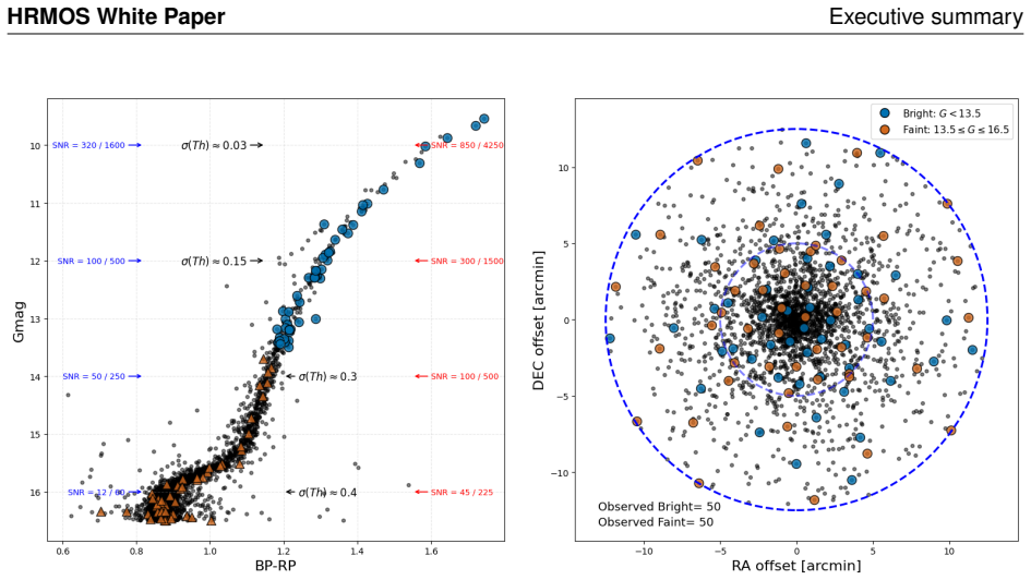
Figure 11.1. Figure 11.1: Two possible telescope pointings of member stars in M67, divided into two G magnitude bins (in orange the faint sample, with 16.5 < G < 13.5, in blue the bright sample, with G < 13.5). The minimum distance between stars within the inner and external regions are 15 arcsec and 30 arcsec, respectively, and the number of allocated fibres is 50 per magnitude bin. In the left panel, the CMD of M67 (stars with… view at source ↗
Figure 11.2
Figure 11.2. Figure 11.2: Spatial distribution of the globular clusters observable with HRMOS, projected onto the Milky Way. The left panel shows the top-down view, while the right panel displays the edge-on view. As a starting point, we compiled potential targets from the Harris Catalogue1 (Harris 2010), which lists 157 Galactic GCs. We selected clusters observable from the Southern hemisphere (DEC < 20◦ ) and with horizontal-b… view at source ↗
Figure 11.3
Figure 11.3. Figure 11.3: Two possible telescope pointings of member stars in NGC6397, divided into two G magnitude bins (in orange the faint sample, with 16.5 < G < 13.5, in blue the bright sample, with G < 13.5). The minimum distance between stars is 30 arcsec, while the number of allocated fibres is 50 per magnitude bin. In the left panel, the CMD of NGC6397 (stars with membership probability > 0.9) is shown. In the right pan… view at source ↗
Figure 11.4
Figure 11.4. Figure 11.4: Upper left: Center of the FOV allocated (blue crosses) in the Sagittarius dwarf galaxy. Upper right: 25 arcmin FOV in the Sagittarius dwarf galaxy, containing at least 100 stars. Lower left: Color–magnitude diagram of one of the fields in the Sagittarius dwarf galaxy. Lower right: Position on the sky of the Sagittarius field with targeted stars in orange symbols. et al. 2023). By adopting an observation… view at source ↗
Figure 11.5
Figure 11.5. Figure 11.5: Upper left: Center of the FOV allocated (blue crosses) in the LMC. Upper right: 25 arcmin FOV in the LMC, containing at least 100 stars. Lower left: Color–magnitude diagram of one of the fields in the LMC. Lower right: Position on the sky of the LMC with targeted stars in orange symbols. providing a solid basis for detailed chemical and kinematic studies of these extended systems. Even a limited set of … view at source ↗
Figure 11.6
Figure 11.6. Figure 11.6: Upper left: Center of the FOV allocated (blue crosses) in the Baade’s window area. Upper right: 25 arcmin FOV in the Baade’s window area. Each of them contains at least 100 stars. Lower left: Color–magnitude diagram of one of the fields in Baade’s window area. Lower right: Position on the sky of the Baade’s window field with targeted stars in orange symbols. 131 [PITH_FULL_IMAGE:figures/full_fig_p133_1… view at source ↗
Figure 12.1
Figure 12.1. Figure 12.1: illustrates the dependence of the abundance uncertainty on the intrinsic abundance and SNR for [Th/Fe], adopting the following stellar parameters: Teff–log g pairs of 5800 K–3.7 dex, 6400 K–4.1 dex, and 6000 K–4.5 dex for dwarf main-sequence stars, and 4800 K–1.2 dex, 5000 K– 2.0 dex, and 5200 K–2.5 dex for red giant branch stars. Microturbulence values of vmic = 1.2 km s−1 and 2.0 km s−1 were adopted f… view at source ↗
Figure 12.2
Figure 12.2. Figure 12.2: Precision in the measurement of La abundances as a function of metallicity and of SNR. Stellar parameters are as in [PITH_FULL_IMAGE:figures/full_fig_p135_12_2.png] view at source ↗
Figure 12.3
Figure 12.3. Figure 12.3: Precision in the measurement of Eu abundances as a function of metallicity and of SNR. Stellar parameters are as in [PITH_FULL_IMAGE:figures/full_fig_p135_12_3.png] view at source ↗
Figure 12.4
Figure 12.4. Figure 12.4: Precision in the measurement of Pb abundances as a function of metallicity and of SNR. Stellar parameters are as in [PITH_FULL_IMAGE:figures/full_fig_p136_12_4.png] view at source ↗
Figure 12.5
Figure 12.5. Figure 12.5: Precision in the measurement of Ba isotopic ratio as a function of metallicity and of SNR. Stellar parameters are as in [PITH_FULL_IMAGE:figures/full_fig_p136_12_5.png] view at source ↗

discussion (0)

Sign in with ORCID, Apple, or X to comment. Anyone can read and Pith papers without signing in.

Forward citations

Cited by 2 Pith papers

Reviewed papers in the Pith corpus that reference this work. Sorted by Pith novelty score.

  1. HRMOS: a very high-resolution, multi-object spectrograph for the ESO VLT

    astro-ph.IM 2026-07 conditional novelty 6.0

    HRMOS is a proposed VLT instrument combining R=80,000 spectroscopy with 50–60 simultaneous fibers and 10 m/s radial-velocity precision across three optical bands.

  2. Stellar Population Astrophysics (SPA) with the TNG. Beyond the iron peak: Galactic evolution of molybdenum, ruthenium and zirconium through open clusters

    astro-ph.GA 2026-07 conditional novelty 5.0

    First large-sample ruthenium abundances in open clusters show Mo and Ru track s-process elements with slopes near unity, while relations with europium deviate, indicating mixed nucleosynthetic sources.

Reference graph

Works this paper leans on

100 extracted references · cited by 2 Pith papers

  1. [1]

    Fermi 5, 50125 Firenze, Italy

    INAF - Osservatorio Astrofisico di Arcetri, Largo E. Fermi 5, 50125 Firenze, Italy

  2. [2]

    Lund Observatory, Division of Astrophysics, Department of Physics, Lund University, Sweden

  3. [3]

    INAF - Osservatorio Astronomico di Brera, Via Bianchi 46, 23807, Merate, Italy

  4. [4]

    UK Astronomy Technology Centre, Edinburgh, United Kingdom

  5. [5]

    Astrofísico Fco

    Facultad de Física, Universidad de La Laguna, Avda. Astrofísico Fco. Sánchez s/n, 38206, La Laguna, Santa Cruz de Tenerife, Spain

  6. [6]

    Vía Làctea, s/n, 38205 La Laguna, Santa Cruz de Tenerife, Spain

    Instituto de Astrofísica de Canarias, C. Vía Làctea, s/n, 38205 La Laguna, Santa Cruz de Tenerife, Spain

  7. [7]

    Instituto de Astrofísica e Ciências do Espaço, Universidade do Porto, CAUP, Rua das Estrelas, 4150-762 Porto, Portugal

  8. [8]

    INAF- Direzione Scientifica- Viale del Parco Mellini, 84, Roma, Italy

  9. [9]

    Departamento de Física e Astronomia, FCUP, Rua do Campo Alegre 687, Porto, Portugal

  10. [10]

    Theoretical Astrophysics, Department of Physics and Astronomy, Uppsala University, Uppsala, Sweden

  11. [11]

    Departamento de Física Teórica, Atómica y Óptica, Universidad de Valladolid, Valladolid, Spain

  12. [12]

    Department of Physics, Imperial College London, London, UK

  13. [13]

    Departament d’Astronomia i Astrofísica, Universitat de València, Burjassot, Spain

  14. [14]

    of Physics, University of Rome Tor Vergata, Rome, Italy

    Dept. of Physics, University of Rome Tor Vergata, Rome, Italy

  15. [15]

    12, 60438, Frankfurt am Main, Germany

    Goethe University Frankfurt, Institute for Applied Physics, Max-von-Laue-Str. 12, 60438, Frankfurt am Main, Germany

  16. [16]

    Observatoire de la Côte d’Azur, Université Côte d’Azur, CNRS, Laboratoire Lagrange, Nice, France

  17. [17]

    Keele University, Keele, ST5 5BG, UK

  18. [18]

    Dipartimento di Fisica e Astronomia, Universita di Bologna, Via Gobetti 93/2, Bologna, Italy

  19. [19]

    INAF - Osservatorio di Astrofisica e Scienza dello Spazio di Bologna, Via Gobetti 93/3, Bologna, Italy

  20. [20]

    INAF - Osservatorio Astronomico di Trieste, via Tiepolo 11, 34143, Trieste, Italy

  21. [21]

    IFPU – Institute for Fundamental Physics of the Universe, via Beirut 2, I-34151 Trieste, Italy

  22. [22]

    Sansone 1, Sesto Fiorentino, Italy [23]NicolausCopernicusAstronomicalCenter, PolishAcademyofSciences, ul

    Dipartimento di Fisica e Astronomia, Universita degli Studi di Firenze, Via G. Sansone 1, Sesto Fiorentino, Italy [23]NicolausCopernicusAstronomicalCenter, PolishAcademyofSciences, ul. Bartycka18, Warsaw, Poland

  23. [23]

    Technische Universität Darmstadt, Department of Physics, 64289 Darmstadt, Germany

  24. [24]

    GSI Helmholtzzentrum für Schwerionenforschung GmbH, 64291 Darmstadt, Germany

  25. [25]

    Max-Planck-Institut für Kernphysik, Saupfercheckweg 1, 69117 Heidelberg, Germany

  26. [26]

    ESO European Southern Observatory, Alonso de Córdova 3107, Vitacura, Santiago, Chile

  27. [27]

    Universidade de São Paulo, IAG, Rua do Matão 1226, São Paulo, Brazil

  28. [28]

    School of Physical Sciences, The Open University, Walton Hall, Milton Keynes, MK7 6AA, UK

  29. [29]

    School of Mathematics and Physics, The University of Queensland, St Lucia, QLD 4072, Australia

  30. [30]

    INAF - Osservatorio Astronomico di Roma, Via Frascati 88, I-00040 Monte Porzio Catone (RM), Italy

  31. [31]

    Enrico Fermi

    Dipartimento di Física “Enrico Fermi”, Università di Pisa, Largo Bruno Pontecorvo 3, Pisa, I-56127, Italy

  32. [32]

    Interdisciplinary Center for Scientific Computing (IWR), University of Heidelberg, Im Neuenheimer Feld 205, 69120, Heidelberg, Germany

  33. [33]

    Universität Heidelberg, Zentrum für Astronomie, Institut für Theoretische Astrophysik, Albert-Ueberle-Strasse 2, 69120, Heidelberg, Germany

  34. [34]

    Australian National University; ARC Centre of Excellence for All Sky Astrophysics in 3 Dimensions 159 HRMOS White PaperAffiliations (ASTRO 3D)

  35. [35]

    Space sciences, Technologies and Astrophysics Research (STAR) Institute, Université de Liège, Liège, Belgium

  36. [36]

    Dipartimento di Fisica, Università degli Studi di Trieste, via Tiepolo 11, 34143, Trieste, Italy

  37. [37]

    SUPA School of Physics and Astronomy, University of St Andrews, North Haugh, St Andrews KY16 9SS, UK

  38. [38]

    Centre for Extragalactic Astronomy, Durham University, South Road, Durham DH1 3LE, UK

  39. [39]

    Department of Physics, Durham University, South Road, Durham DH1 3LE, UK

  40. [40]

    INAF, Osservatorio Astronomico d’Abruzzo, Via Mentore Maggini Snc, 64100 Teramo, Italy

  41. [41]

    Sezione di Perugia, Istituto Nazionale di Fisica Nucleare, Perugia, Italy

  42. [42]

    INAF - Osservatorio Astronomico di Palermo G.S.Vaiana, Piazza del Parlamento 1, 90134, Palermo, Italy

  43. [43]

    3, 10257 Vilnius, Lithuania

    Vilnius University, Faculty of Physics, Institute of Theoretical Physics and Astronomy, Sauletekio av. 3, 10257 Vilnius, Lithuania

  44. [44]

    Sofia, 78, 95128, Catania, Italy

    INAF - Osservatorio Astrofisico di Catania, via S. Sofia, 78, 95128, Catania, Italy

  45. [45]

    Lluis Companys 28, E-08010 Barcelona, Spain; Institut de Ciencies del Cosmos (ICCUB), Universitat de Barcelona (UB), c

    ICREA, Pg. Lluis Companys 28, E-08010 Barcelona, Spain; Institut de Ciencies del Cosmos (ICCUB), Universitat de Barcelona (UB), c. Marti i Franques, 1, E-08028 Barcelona, Spain

  46. [46]

    Institut d’Estudis Espacials de Catalunya (IEEC), Edifici RDIT, Campus UPC, E-08860 Castelldefels (Barcelona), Spain

  47. [47]

    Department of Physics and Astronomy, University of Notre Dame, 225 Nieuwland Science Hall, Notre Dame, IN 46556, USA

  48. [48]

    Department of Physics, University of Warwick, Gibbet Hill Road, Coventry CV4 7AL, UK

  49. [49]

    Centre for Exoplanets and Habitability, University of Warwick, Gibbet Hill Road, Coventry CV4 7AL, UK

  50. [50]

    Laboratoire d’Astrophysique de Bordeaux, Université Bordeaux, CNRS, B18N, Allée Geoffroy Saint-Hilaire, 33615, Pessac, France

  51. [51]

    Galileo Galilei

    Dipartimento di Fisica e Astronomia "Galileo Galilei", Università degli Studi di Padova, Vicolo dell’Osservatorio 3, 35122 Padova, Italy

  52. [52]

    Astronomisches Rechen-Institut, Zentrum für Astronomie der Universität Heidelberg, Mönchhofstraße 12-14, 69120, Heidelberg, Germany

  53. [53]

    Institut d’Astronomie et d’Astrophysique, Université Libre de Bruxelles (ULB), CP 226, Boulevard du Triomphe, 1050, Bruxelles, Belgium

  54. [54]

    Royal Observatory of Belgium, Avenue Circulaire 3, 1180 Brussels, Belgium

  55. [55]

    Space Telescope Science Institute

  56. [56]

    INAF - Osservatorio Astronomico di Padova, Vicolo dell’Osservatorio 5, 85122, Padova, Italy

  57. [57]

    INAF - Osservatorio Astrofisico di Torino, Via Osservatorio 20, 10025, Pino Torinese (TO), Italy

  58. [58]

    ut 15-17, Hungary

    HUN REN Konkoly Observatory, CSFK, H-1121, Budapest, Konkoly Thege M. ut 15-17, Hungary

  59. [59]

    CSFK, MTA Centre of Excellence, Budapest, Konkoly Thege Miklos ut 15-17, H-1121, Hungary

  60. [60]

    University of Bayreuth, BGI, Universitatsstrasse 30, 95447 Bayreuth, Germany

  61. [61]

    Heidelberger Institut für Theoretische Studien, Schloss-Wolfsbrunnenweg 35, D-69118 Heidelberg, Germany

  62. [62]

    European Space Agency (ESA), European Space Astronomy Centre (ESAC), Camino Bajo del Castillo s/n, E-28692 Villanueva de la Cañada, Madrid, Spain

  63. [63]

    Department of Astronomy, The Ohio State University, Columbus, OH 43210, USA

  64. [64]

    Center for Cosmology and AstroParticle Physics (CCAPP), The Ohio State University, Columbus, OH 160 HRMOS White PaperAffiliations 43210, USA

  65. [65]

    Max-Planck-Institut für Astronomie, Königstuhl 17, D-69117 Heidelberg, Germany

  66. [66]

    University of Victoria (Canada)

  67. [67]

    School of Physical and Chemical Sciences - Te Kura Matu, University of Canterbury, Private Bag 4800, Christchurch, 8140, New Zealand

  68. [68]

    Centre for Astrophysics Research, University of Hertfordshire, Hatfield, AL10 9AB, UK

  69. [69]

    Department of Physics, University of Surrey, Stag Hill, Guildford, GU2 7XH, UK

  70. [70]

    Department of Astrophysics, University of Vienna, Turkenschanzstrasse 17, 1180, Vienna

  71. [71]

    University of Southern Queensland

  72. [72]

    Research School of Astronomy and Astrophysics, The Australian National University, Canberra, ACT 2611, Australia

  73. [73]

    Centro de Astrobiología (CAB), CSIC-INTA, Camino Bajo del Castillo s/n, 28692, Villanueva de la Cañada (Madrid), Spain

  74. [74]

    Vicuña Mackenna 4860, Macul, Santiago, 7820436, Chile

    Instituto de Astrofísica, Facultad de Física, Pontificia Universidad Católica de Chile, Campus San Joaquín, Av. Vicuña Mackenna 4860, Macul, Santiago, 7820436, Chile

  75. [75]

    INAF-IAPS, Via del Fosso del Cavaliere 100, Roma, Italy

  76. [76]

    Purple Mountain Observatory, Chinese Academy of Sciences, Nanjing, 210023, PR China

  77. [77]

    Department of Astronomy, Stockholm University, AlbaNova University Centre, Stockholm, Sweden

  78. [78]

    Materials Science and Applied Mathematics, Mälmö University, 20506, Mälmö, Sweden

  79. [79]

    Department of Astronomy, The University of Texas at Austin, 2515 Speedway Boulevard, Austin, TX 78712, USA

  80. [80]

    Institut d’astrophysique de Paris, CNRS

Showing first 80 references.

This paper was first reviewed by grok-4.5 on July 11, 2026.