Quantized tensor networks for solving the Vlasov-Maxwell equations
Pith reviewed 2026-05-24 05:35 UTC · model grok-4.3
The pith
Quantized tensor networks solve five-dimensional Vlasov-Maxwell problems at a bond dimension of 64 instead of 2^18.
A machine-rendered reading of the paper's core claim, the machinery that carries it, and where it could break.
Core claim
The central claim is that the quantized tensor network (QTN) representation reduces the cost of grid-based Vlasov-Maxwell simulation from O(N) to O(poly(D)), and that a modest bond dimension D=64 is already sufficient to capture the expected physics in five-dimensional test problems whose full-rank equivalent would require D=2^18.
What carries the argument
The quantized tensor network (QTN) representation of the distribution function and fields, compressed to low bond dimension D.
If this is right
- Five-dimensional Vlasov-Maxwell simulations with 2^36 grid points become practical at modest computational cost.
- The Dirac-Frenkel variational time evolution permits stable steps exceeding the CFL limit.
- Full-rank storage and arithmetic at D equal to half the number of grid points are unnecessary for these problems.
- The same compression applies to both the distribution function and the self-consistent electromagnetic fields.
Where Pith is reading between the lines
- If the low-rank property persists across a broader class of initial conditions, the method could be applied to other high-dimensional kinetic models without major reformulation.
- The same QTN structure might allow direct comparison of reduced-cost runs against analytic limits in regimes where full-grid verification remains impossible.
- Extensions to six-dimensional problems would become feasible provided the required bond dimension stays well below the exponential growth of the grid size.
Load-bearing premise
The physical solutions of the Vlasov-Maxwell system for the test problems admit an accurate low-rank representation in the quantized tensor network format at D=64.
What would settle it
A side-by-side run in which the D=64 QTN solution produces instability growth rates or final particle distributions that deviate measurably from those obtained with a converged full-grid or higher-D reference calculation on the same test problem.
Figures




read the original abstract
The Vlasov-Maxwell equations provide an \textit{ab-initio} description of collisionless plasmas, but solving them is often impractical because of the wide range of spatial and temporal scales that must be resolved and the high dimensionality of the problem. In this work, we present a quantum-inspired semi-implicit Vlasov-Maxwell solver that utilizes the quantized tensor network (QTN) framework. With this QTN solver, the cost of grid-based numerical simulation of size $N$ is reduced from $\mathcal{O}(N)$ to $\mathcal{O}(\text{poly}(D))$, where $D$ is the ``rank'' or ``bond dimension'' of the QTN and is typically set to be much smaller than $N$. We find that for the five-dimensional test problems considered here, a modest $D=64$ appears to be sufficient for capturing the expected physics despite the simulations using a total of $N=2^{36}$ grid points, \edit{which would require $D=2^{18}$ for full-rank calculations}. Additionally, we observe that a QTN time evolution scheme based on the Dirac-Frenkel variational principle allows one to use somewhat larger time steps than prescribed by the Courant-Friedrichs-Lewy (CFL) constraint. As such, this work demonstrates that the QTN format is a promising means of approximately solving the Vlasov-Maxwell equations with significantly reduced cost.
Editorial analysis
A structured set of objections, weighed in public.
Referee Report
Summary. The manuscript presents a quantized tensor network (QTN) framework for solving the five-dimensional Vlasov-Maxwell equations, reducing the computational cost of an N=2^36 grid from O(N) to O(poly(D)) with bond dimension D=64 claimed to be sufficient for capturing the expected physics in the considered test problems; it further reports that a Dirac-Frenkel variational time-evolution scheme permits time steps exceeding the CFL limit.
Significance. If the low-rank QTN representation is shown to incur controllable truncation error, the method would offer a promising route to mitigating the curse of dimensionality in ab-initio collisionless plasma simulations; the work supplies a concrete demonstration on 5D test problems and identifies a variational integrator that relaxes the CFL constraint.
major comments (2)
- [Abstract] Abstract and results sections: the central claim that D=64 'appears to be sufficient for capturing the expected physics' for N=2^36 grids is load-bearing yet unsupported by explicit quantitative metrics; no L2 or other error norms versus a reference solution, no convergence tables of diagnostics versus D, and no comparison against full-rank or higher-D runs are reported, leaving open the possibility that truncation error is masked by the smoothness of the test cases or by the chosen observables.
- [Time evolution] Section on time evolution (Dirac-Frenkel scheme): the observation that the variational integrator allows time steps larger than the CFL limit requires supporting evidence such as stability diagrams, error-versus-dt plots, or direct comparison against a CFL-compliant reference integrator; without these, the claim remains qualitative and does not establish the practical advantage.
minor comments (2)
- [Methods] Notation for the quantized tensor-train format and the mapping from the five-dimensional phase-space grid to the QTN indices should be introduced with an explicit diagram or equation early in the methods section to aid reproducibility.
- [Test problems] The manuscript should state the precise form of the Vlasov-Maxwell system (including normalization and boundary conditions) used in the test problems so that the reported physics can be independently verified.
Simulated Author's Rebuttal
We thank the referee for their careful reading of the manuscript and for the constructive comments. We address each major point below and will revise the manuscript to incorporate additional quantitative evidence.
read point-by-point responses
-
Referee: [Abstract] Abstract and results sections: the central claim that D=64 'appears to be sufficient for capturing the expected physics' for N=2^36 grids is load-bearing yet unsupported by explicit quantitative metrics; no L2 or other error norms versus a reference solution, no convergence tables of diagnostics versus D, and no comparison against full-rank or higher-D runs are reported, leaving open the possibility that truncation error is masked by the smoothness of the test cases or by the chosen observables.
Authors: We agree that the sufficiency of D=64 requires stronger quantitative support. The present manuscript demonstrates agreement with expected physical behavior on standard 5D test problems but does not report explicit L2 norms or systematic convergence with D. In the revised version we will add L2 error norms of the distribution function and fields against reference solutions (where computable at lower resolution), together with tables of diagnostic convergence (energy conservation, growth rates) versus D up to at least 128. These additions will directly address the possibility of masked truncation error. revision: yes
-
Referee: [Time evolution] Section on time evolution (Dirac-Frenkel scheme): the observation that the variational integrator allows time steps larger than the CFL limit requires supporting evidence such as stability diagrams, error-versus-dt plots, or direct comparison against a CFL-compliant reference integrator; without these, the claim remains qualitative and does not establish the practical advantage.
Authors: We acknowledge that the statement concerning time steps larger than the CFL limit is currently qualitative. The revised manuscript will include error-versus-dt plots for representative test problems, showing both global error and conservation properties as dt is increased beyond the CFL limit, together with direct comparisons against a standard explicit integrator run at CFL-compliant steps. These figures will quantify the practical advantage of the Dirac-Frenkel scheme. revision: yes
Circularity Check
No significant circularity detected
full rationale
The paper presents a new QTN-based numerical solver for the Vlasov-Maxwell system and supports its claims via direct numerical experiments on five-dimensional test problems. No derivation step reduces by construction to its own inputs: the reported sufficiency of D=64 is an empirical observation from the simulations rather than a fitted parameter renamed as a prediction, and no load-bearing uniqueness theorem or ansatz is imported via self-citation. The method is self-contained against external benchmarks (standard Vlasov-Maxwell test cases) with no evidence of self-definitional or fitted-input circularity.
Axiom & Free-Parameter Ledger
free parameters (1)
- bond dimension D =
64
axioms (1)
- domain assumption Solutions to the Vlasov-Maxwell equations can be accurately approximated by low bond-dimension quantized tensor networks for the test cases considered.
Forward citations
Cited by 2 Pith papers
-
Quantum-Inspired Simulation of 2D Turbulent Rayleigh-B\'enard Convection
Matrix product state simulations of 2D Rayleigh-Bénard convection recover Nusselt number statistics with 1.8% error and a 9-fold reduction in degrees of freedom at Ra=10^10 using bond dimensions comparable to lower Ra cases.
-
Quantum-Inspired Tensor-Network Fractional-Step Method for Incompressible Flow in Curvilinear Coordinates
Tensor-network fractional-step method simulates incompressible flows in curvilinear coordinates with up to 20x field compression and 1000x operator compression while keeping errors below 0.3% versus finite differences.
Reference graph
Works this paper leans on
-
[1]
QTT-Operator for first derivative The QTT-Operator for the first derivative along one axis can be written explicitly, assuming uniform grid points and a finite difference scheme. With periodic boundary conditions and a centered second-order stencil, it is ∂ ∂x≈1 ∆x [I S+ +S−S+ +S−] I S−S+ 0 S+ 0 0 0 S− I S−S+ 0 S+ 0 0 0 S− ... I S−S+ 0 ...
-
[2]
Application of QTT-Operators to QTTs Example 1. As a brief aside, consider a system with 8 grid points and suppose our vector of interest is all ones. The corresponding QTT is rank 1, and given by h = [1, 1, 1, 1, 1, 1, 1, 1]∼= 1⊗1⊗1 = [1][1][1] where 1 = [ 1 1 ] . Applying the finite difference operator in Eq. (3) to this QTT, we obtain the following QTT...
-
[3]
Element-wise Multiplication The Vlasov equation also requires performing elemental multiplication of generic functions h1(x)h2(x). This com- putation is performed by writingh1(x) as a diagonal matrix andh2(x) as a vector, and then performing matrix-vector multiplication. For the spatial advection term, we require diagonalizing h1(v) = v. Analogous to Eq. ...
-
[4]
Multi-dimensional operators While the operators in the above discussion act only on one dimension, they can still be represented in a multi- dimensional space. To do this, one simply pads the original QTT with a tensor train of identity matrices for the remaining dimensions. For example, for a 2-D system with dimensions along x and v, if a sequential orde...
-
[5]
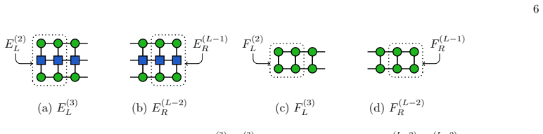
Tensor train geometry Let us consider tensor trains of length L. In this case, the left or right environments for ⟨b|A|x⟩are (see Fig 1(a) and (b)) (E(p) L )αbp,αAp,αxp = ∑ αb p−1,αA p−1,αx p−1 ∑ op,ip B(p)∗ αb p−1,αbp (op)A(p) αA p−1,αAp (op,ip)X(p) αx p−1,αxp (ip)(E(p−1) L )αb p−1,αA p−1,αx p−1 , (16) (E(p) R )αb p−1,αA p−1,αx p−1 = ∑ αbp,αAp,αxp ∑ op,i...
-
[6]
The primary difference lies in contracting the tensor along the spine
Comb geometry For a comb tensor network with K branches, one first computes the environments starting from the ends of the branch as described above, obtaining the right environments {E(k) R,branch}. The primary difference lies in contracting the tensor along the spine. Again, for concreteness, let us consider the expectation value ⟨b|A|x⟩. In this case t...
-
[7]
First is to build the left or right environments for ⟨x|A|x⟩and for ⟨x|b⟩. Again, the environments are gener- ally built recursively because each are also used to compute A(p,p+1) eff and b(p,p+1) eff . The cost of building the environment scales likeO(D3 xDAd +D2 xD2 Ad2)
-
[8]
The second step is to update the tensors in |x⟩by solving Eq. (31) as described above, starting with sites 1 and 2 of the QTT and then sweeping left to right through the chain of tensors. In this case, one only needs to first build the right environments. After updating sites p andp + 1, one computes new left environments EL,(p) and FL,(p) as depicted in ...
-
[9]
At the end of each sweep, one computes the error ||b−Ax||2. If the error is still too large, one continues to the next iteration, sweeping in the opposite direction. By computing the error as ⟨b|b⟩−2⟨b|A|x⟩+⟨x|A†A|x⟩, the cost typically is dominated by the last term, which scales like O(2D3 xD2 Ad + 2D2 xD3 Ad2). One could consider a less exact measure of...
-
[10]
Results for calculations with QTC geometry The electric and magnetic (EM) fields for simulations of the Orszag-Tang vortex performed with bond dimension D = 64 and time step ∆ t = 0.001Ω−1 c,p are shown in Fig. 8. As mentioned in the main text, the electric fields appear to be the primary source of noise. FIG. 8. Each component of the magnetic (top) and e...
-
[11]
Entanglement entropy for different QTN ansatz¨ e In Fig. 11, we measure the entanglement entropy at each bond for three different geometries: • the QTC geometry with flipped binary mapping for each axis (presented in the main paper). • QTT-SFB: QTT geometry with sequential ordering, with binary mapping for position axes and flipped binary mapping for velo...
-
[12]
In the case that α= 1/2, one obtains the Crank-Nicolson scheme
Calculations with uncentered Crank-Nicolson Single-step time integration schemes can generally be written as ϕn+1−ϕn ∆t = (1−α)F(ϕn,tn) +αF(ϕn+1,tn+1), (40) where ϕn is the solution and F(ϕn,tn) is the time derivative of ϕat time tn. In the case that α= 1/2, one obtains the Crank-Nicolson scheme. The time integration scheme is stable for α≥0.5 [17]. In Fi...
-
[13]
Observed scalings of cost with respect to QTN bond dimension The wall-time of the real-space and velocity-space advection steps are measured with respect to QTN bond dimension D for the Orszag-Tang problem. (Since the velocity-space advection step is performed twice per actual time step, the plotted value is those two times averaged together.) The wall-ti...
-
[14]
Schollw¨ ock, The density-matrix renormalization group in the age of matrix product states, Ann
U. Schollw¨ ock, The density-matrix renormalization group in the age of matrix product states, Ann. Phys.326, 96 (2011)
work page 2011
-
[15]
Institute, Resources for tensor network algorithms, theory, and software (2023)
F. Institute, Resources for tensor network algorithms, theory, and software (2023)
work page 2023
-
[16]
J. J. G. Ripoll, Quantum-inspired algorithms for multivariate analysis: from interpolation to partial differential equation, Quantum 5, 431 (2021)
work page 2021
-
[17]
I. V. Oseledets, Tensor-train decomposition, SIAM J. Sci. Comput. 33, 2295 (2011)
work page 2011
-
[18]
E. M. Stoudenmire and S. R. White, Minimally entangled typical thermal state algorithms, New J. Phys. 12, 055026 (2010)
work page 2010
- [19]
-
[20]
I. P. McCulloch, From density-matrix renormalization group to matrix product states, J. Stat. Mech. , P10014 (2007)
work page 2007
-
[21]
J. Haegeman, C. Lubich, I. Oseledets, B. Vandereycken, and F. Verstraete, Unifying time evolution and optimization with matrix product states, Phys. Rev. B 94, 165116 (2016)
work page 2016
-
[22]
S. Paeckel, T. K¨ ohler, A. Swoboda, S. R. Manmana, U. Schollw¨ ock, and C. Hubig, Time-evolution methods for matrix- product states, Ann. Phys. 411, 167998 (2019)
work page 2019
-
[23]
D. Bauernfeind and M. Aichhorn, Time dependent variational principle for tree tensor networks, 8, 024 (2020)
work page 2020
-
[24]
S. V. Dolgov, B. N. Khoromskij, I. V. Oseledets, and D. V. Savostyanov, Computation of extreme eigenvalues in higher dimensions using block tensor train format, Comput. Phys. Commun. 185, 1207 (2014)
work page 2014
-
[25]
I. V. Oseledets and S. V. Dolgov, Solution of linear systems and matrix inversion in the TT-format, SIAM J. Sci. Comput. 34, A2718 (2012)
work page 2012
-
[26]
S. V. Dolgov and D. V. Savostyanov, Alternating minimal energy method for linear systems in higher dimensions, SIAM J. Sci. Comput 36, A2248 (2014)
work page 2014
-
[27]
J. R. Shewchuk, An Introduction to the Conjugate Gradient Method Without the Agonizing Pain , Tech. Rep. (Pittsburgh, PA, 1994)
work page 1994
-
[28]
Sonneveld, CGS, A fast Lanczos-type solver for nonsymmetric linear systems, SIAM J
P. Sonneveld, CGS, A fast Lanczos-type solver for nonsymmetric linear systems, SIAM J. Sci. Stat. Comp. 10, 36 (1989)
work page 1989
-
[29]
N. Gourianov, M. Lubasch, S. Dolgov, et al. , A quantum inspired approach to exploit turbulence structures, Nature Comput. Sci. 2, 30 (2022)
work page 2022
-
[30]
D. R. Durran, Numerical Methods for Fluid Dynamics: With Applications to Geophysics (Springer, 2010)
work page 2010
discussion (0)
Sign in with ORCID, Apple, or X to comment. Anyone can read and Pith papers without signing in.