Time-optimal Convexified Reeds-Shepp Paths on a Sphere
Pith reviewed 2026-05-22 21:43 UTC · model grok-4.3
The pith
Time-optimal paths for a convexified Reeds-Shepp vehicle on a sphere consist of at most six segments from three motion primitives.
A machine-rendered reading of the paper's core claim, the machinery that carries it, and where it could break.
Core claim
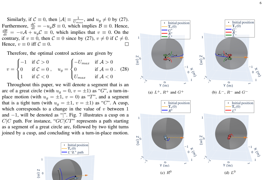
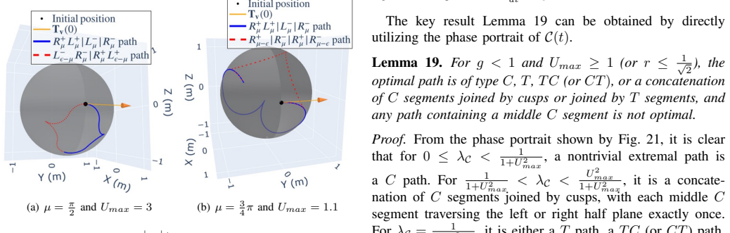
Using Pontryagin's Maximum Principle and a phase-portrait analysis, the optimal path connecting a given initial configuration to a desired terminal configuration consists of at most six segments drawn from three motion primitives: tight turns, great circular arcs, and turn-in-place motions. A complete classification yields a finite sufficient list of 23 optimal path types with closed-form segment angles derived.
What carries the argument
Pontryagin's Maximum Principle applied to derive extremal trajectories, followed by phase-portrait analysis to classify switches between motion primitives.
If this is right
- The global optimum can always be found by checking only the 23 candidate path types.
- Each of the 23 types has closed-form expressions for its segment angles.
- The same structure applies to underactuated satellite attitude control and spherical rolling robots.
- Turning-rate bounds below 1 are handled by an equivalent reformulation of the problem.
Where Pith is reading between the lines
- The finite list of 23 types could support a discrete graph search for real-time planning on spheres.
- Similar phase-portrait methods might classify optimal paths on other constant-curvature surfaces.
- The closed-form solutions provide exact benchmarks for testing numerical optimal-control solvers.
Load-bearing premise
The phase-portrait analysis and PMP application fully capture all extremal trajectories without additional singular cases or missed switches for the spherical geometry when the turning-rate bound is at least 1.
What would settle it
A pair of initial and terminal configurations whose time-optimal path requires more than six segments or a motion primitive outside the three listed would show the classification is incomplete.
Figures





read the original abstract
This article studies the time-optimal path planning problem for a convexified Reeds-Shepp (CRS) vehicle on a unit sphere, capable of both forward and backward motion, with speed bounded in magnitude by 1 and turning rate bounded in magnitude by a given constant. For the case in which the turning-rate bound is at least 1, using Pontryagin's Maximum Principle and a phase-portrait analysis, we show that the optimal path connecting a given initial configuration to a desired terminal configuration consists of at most six segments drawn from three motion primitives: tight turns, great circular arcs, and turn-in-place motions. A complete classification yields a finite sufficient list of 23 optimal path types with closed-form segment angles derived. The complementary case in which the turning-rate bound is less than 1 is addressed via an equivalent reformulation. The proposed formulation is applicable to underactuated satellite attitude control, spherical rolling robots, and mobile robots operating on spherical or gently curved surfaces. The source code for solving the time-optimal path problem and visualization is publicly available at https://github.com/sixuli97/Optimal-Spherical-Convexified-Reeds-Shepp-Paths.
Editorial analysis
A structured set of objections, weighed in public.
Referee Report
Summary. This paper studies the time-optimal path planning problem for a convexified Reeds-Shepp (CRS) vehicle on a unit sphere, with speed bounded in magnitude by 1 and turning rate bounded by a constant κ. For the case κ ≥ 1, Pontryagin's Maximum Principle combined with phase-portrait analysis is used to prove that any optimal path consists of at most six segments drawn from three primitives (tight turns, great circular arcs, turn-in-place motions). A complete classification produces a finite list of 23 admissible path types together with closed-form expressions for the segment angles. The case κ < 1 is handled by an equivalent reformulation. The formulation targets applications in underactuated satellite attitude control and spherical rolling robots; public code is provided.
Significance. If the classification and closed-form derivations hold, the work supplies a complete, finite catalogue of time-optimal trajectories for this nonholonomic system on the sphere, directly extending the classical Reeds-Shepp result to spherical geometry. The explicit list of 23 word types and the public repository constitute a practical, reproducible contribution that can be used for real-time planning in satellite and mobile-robot applications.
minor comments (1)
- The abstract states that the source code is publicly available; the manuscript would benefit from an explicit citation of the repository in the main text (e.g., in the introduction or conclusion) so that readers can locate the implementation without searching the abstract.
Simulated Author's Rebuttal
We thank the referee for their positive assessment of the manuscript, including the detailed summary of our contributions and the recommendation to accept. No major comments requiring response or revision were raised.
Circularity Check
No significant circularity
full rationale
The paper's central derivation applies Pontryagin's Maximum Principle (a standard external theorem) to the spherical control system and performs a phase-portrait analysis to enumerate extremals, yielding the 23 path types and closed-form angles. These steps rely on established optimal-control machinery and geometric properties of the sphere rather than any self-definition, fitted inputs renamed as predictions, or load-bearing self-citations. The restriction to turning-rate bound ≥1 is an explicit modeling choice, and the complementary case is handled by reformulation; no equation reduces to its own input by construction. The public code further supports independent verification outside the paper.
Axiom & Free-Parameter Ledger
axioms (2)
- standard math Pontryagin's Maximum Principle can be applied to characterize the time-optimal trajectories
- domain assumption The phase-portrait analysis on the sphere covers all possible switching sequences without missed cases
Reference graph
Works this paper leans on
-
[1]
Time-optimal trajectories for an omni-directional vehicle,
D. J. Balkcom, P. A. Kavathekar, and M. T. Mason, “Time-optimal trajectories for an omni-directional vehicle,” The International Journal of Robotics Research , vol. 25, no. 10, pp. 985–999, 2006
work page 2006
-
[2]
Maneuver-based motion planning for nonlinear systems with symmetries,
E. Frazzoli, M. A. Dahleh, and E. Feron, “Maneuver-based motion planning for nonlinear systems with symmetries,” IEEE transactions on robotics, vol. 21, no. 6, pp. 1077–1091, 2005
work page 2005
-
[3]
A computationally ef- ficient motion primitive for quadrocopter trajectory generation,
M. W. Mueller, M. Hehn, and R. D’Andrea, “A computationally ef- ficient motion primitive for quadrocopter trajectory generation,” IEEE transactions on robotics , vol. 31, no. 6, pp. 1294–1310, 2015
work page 2015
-
[4]
L. E. Dubins, “On curves of minimal length with a constraint on average curvature, and with prescribed initial and terminal positions and tangents,”American Journal of mathematics, vol. 79, no. 3, pp. 497–516, 1957
work page 1957
-
[5]
Optimal paths for a car that goes both forwards and backwards,
J. Reeds and L. Shepp, “Optimal paths for a car that goes both forwards and backwards,” Pacific journal of mathematics , vol. 145, no. 2, pp. 367–393, 1990
work page 1990
-
[6]
L. S. Pontryagin, Mathematical theory of optimal processes. Routledge, 2018
work page 2018
-
[7]
Shortest paths of bounded curvature in the plane,
J.-D. Boissonnat, A. C ´er´ezo, and J. Leblond, “Shortest paths of bounded curvature in the plane,” Journal of Intelligent and Robotic Systems , vol. 11, pp. 5–20, 1994
work page 1994
-
[8]
H. J. Sussmann and G. Tang, “Shortest paths for the reeds-shepp car: a worked out example of the use of geometric techniques in nonlinear optimal control,” Rutgers Center for Systems and Control Technical Report, vol. 10, pp. 1–71, 1991
work page 1991
-
[9]
Minimum wheel-rotation paths for differential-drive mobile robots,
H. Chitsaz, S. M. LaValle, D. J. Balkcom, and M. T. Mason, “Minimum wheel-rotation paths for differential-drive mobile robots,” The Interna- tional Journal of Robotics Research , vol. 28, no. 1, pp. 66–80, 2009
work page 2009
-
[10]
Markov–dubins path via optimal control theory,
C. Y . Kaya, “Markov–dubins path via optimal control theory,” Com- putational Optimization and Applications , vol. 68, no. 3, pp. 719–747, 2017
work page 2017
-
[11]
Non-euclidean dubins’ problem,
F. Monroy-P ´erez, “Non-euclidean dubins’ problem,” Journal of dynam- ical and control systems , vol. 4, pp. 249–272, 1998
work page 1998
-
[12]
The weighted markov-dubins problem,
D. P. Kumar, S. Darbha, S. G. Manyam, and D. Casbeer, “The weighted markov-dubins problem,” IEEE Robotics and Automation Letters, vol. 8, no. 3, pp. 1563–1570, 2023
work page 2023
-
[13]
Time optimal trajectories for bounded velocity differential drive vehicles,
D. J. Balkcom and M. T. Mason, “Time optimal trajectories for bounded velocity differential drive vehicles,” The International Journal of Robotics Research , vol. 21, no. 3, pp. 199–217, 2002
work page 2002
-
[14]
Time optimal trajectories for a car- like mobile robot,
J. Z. Ben-Asher and E. D. Rimon, “Time optimal trajectories for a car- like mobile robot,” IEEE Transactions on Robotics , vol. 38, no. 1, pp. 421–432, 2021
work page 2021
-
[15]
Shortest 3-dimensional paths with a prescribed curva- ture bound,
H. J. Sussmann, “Shortest 3-dimensional paths with a prescribed curva- ture bound,” in Proceedings of 1995 34th IEEE Conference on Decision and Control, vol. 4. IEEE, 1995, pp. 3306–3312
work page 1995
-
[16]
Time-optimal paths for a dubins airplane,
H. Chitsaz and S. M. LaValle, “Time-optimal paths for a dubins airplane,” in 2007 46th IEEE conference on decision and control. IEEE, 2007, pp. 2379–2384
work page 2007
-
[17]
Dubins’ problem on surfaces. i. nonnega- tive curvature,
Y . Chitour and M. Sigalotti, “Dubins’ problem on surfaces. i. nonnega- tive curvature,”The Journal of Geometric Analysis, vol. 15, pp. 565–587, 2005
work page 2005
-
[18]
Optimal geodesic curvature constrained dubins’ paths on a sphere,
S. Darbha, A. Pavan, R. Kumbakonam, S. Rathinam, D. W. Casbeer, and S. G. Manyam, “Optimal geodesic curvature constrained dubins’ paths on a sphere,” Journal of Optimization Theory and Applications , vol. 197, no. 3, pp. 966–992, 2023
work page 2023
-
[19]
D. P. Kumar, S. Darbha, S. G. Manyam, and D. Casbeer, “Generalization of optimal geodesic curvature constrained dubins’ path on sphere with free terminal orientation,” IEEE Control Systems Letters , 2024
work page 2024
-
[20]
Position and attitude control of an underactuated satellite with constant thrust,
Y . Yoshimura, T. Matsuno, and S. Hokamoto, “Position and attitude control of an underactuated satellite with constant thrust,” in AIAA Guidance, Navigation, and Control Conference , 2011, p. 6352
work page 2011
-
[21]
Control of underactuated spacecraft with bounded inputs,
P. Tsiotras and J. Luo, “Control of underactuated spacecraft with bounded inputs,” Automatica, vol. 36, no. 8, pp. 1153–1169, 2000
work page 2000
-
[22]
H. Krishnan, M. Reyhanoglu, and H. McClamroch, “Attitude stabi- lization of a rigid spacecraft using two control torques: A nonlinear control approach based on the spacecraft attitude dynamics,”Automatica, vol. 30, no. 6, pp. 1023–1027, 1994
work page 1994
-
[23]
P. Crouch, “Spacecraft attitude control and stabilization: Applications of geometric control theory to rigid body models,” IEEE Transactions on Automatic Control, vol. 29, no. 4, pp. 321–331, 1984
work page 1984
-
[24]
Control on the sphere and reduced attitude stabilization,
F. Bullo, R. M. Murray, and A. Sarti, “Control on the sphere and reduced attitude stabilization,” IFAC Proceedings Volumes, vol. 28, no. 14, pp. 495–501, 1995
work page 1995
-
[25]
R. M. Murray, Z. Li, and S. S. Sastry, A mathematical introduction to robotic manipulation. CRC press, 2017
work page 2017
-
[26]
Spherical rolling robots—design, modeling, and control: A systematic literature review,
A. Diouf, B. Belzile, M. Saad, and D. St-Onge, “Spherical rolling robots—design, modeling, and control: A systematic literature review,” Robotics and Autonomous Systems , p. 104657, 2024
work page 2024
-
[27]
Motion control of a spherical mobile robot,
A. Halme, T. Schonberg, and Y . Wang, “Motion control of a spherical mobile robot,” in Proceedings of 4th IEEE International Workshop on Advanced Motion Control-AMC’96-MIE, vol. 1. IEEE, 1996, pp. 259– 264
work page 1996
-
[28]
A. Bicchi, A. Balluchi, D. Prattichizzo, and A. Gorelli, “Introducing the” sphericle”: an experimental testbed for research and teaching in nonholonomy,” in Proceedings of International Conference on Robotics and Automation, vol. 3. IEEE, 1997, pp. 2620–2625
work page 1997
-
[29]
Design, analysis and experiments of an omni-directional spherical robot,
Q. Zhan, Y . Cai, and C. Yan, “Design, analysis and experiments of an omni-directional spherical robot,” in 2011 IEEE International Conference on Robotics and Automation . IEEE, 2011, pp. 4921–4926
work page 2011
-
[30]
Spherical robots for special purposes: a review on current possibilities,
M. Buj ˇn´ak, R. Pirn ´ık, K. R ´astoˇcn`y, A. Janota, D. Nemec, P. Kuch ´ar, T. Tich `y, and Z. Łukasik, “Spherical robots for special purposes: a review on current possibilities,” Sensors, vol. 22, no. 4, p. 1413, 2022
work page 2022
-
[31]
Weld line recognition and path planning with spherical tank inspection robots,
J. Li, S. Jin, C. Wang, J. Xue, and X. Wang, “Weld line recognition and path planning with spherical tank inspection robots,” Journal of Field Robotics, vol. 39, no. 2, pp. 131–152, 2022
work page 2022
-
[32]
Development of an autonomous robot for gas storage spheres inspection,
J. Okamoto, V . Grassi, P. F. S. Amaral, B. G. M. Pinto, D. Pipa, G. P. Pires, and M. V . M. Martins, “Development of an autonomous robot for gas storage spheres inspection,” Journal of Intelligent & Robotic Systems, vol. 66, pp. 23–35, 2012
work page 2012
-
[33]
Geomorpho- logical map of the crotone province (calabria, south italy),
F. Luca, G. Robustelli, M. Conforti, and D. Fabbricatore, “Geomorpho- logical map of the crotone province (calabria, south italy),” Journal of Maps, vol. 7, no. 1, pp. 375–390, 2011
work page 2011
-
[34]
Compositional divergence and convergence in local communities and spatially structured landscapes,
T. Caruso, J. R. Powell, and M. C. Rillig, “Compositional divergence and convergence in local communities and spatially structured landscapes,” PLoS One, vol. 7, no. 4, p. e35942, 2012
work page 2012
-
[35]
Equivalence of dubins path on sphere with geographic coordinates and moving frames,
D. P. Kumar, S. Darbha, S. G. Manyam, D. W. Casbeer, and M. Pachter, “Equivalence of dubins path on sphere with geographic coordinates and moving frames,” Journal of Guidance, Control, and Dynamics , pp. 1–6, 2024. 18
work page 2024
-
[36]
Jurdjevic, Geometric control theory
V . Jurdjevic, Geometric control theory . Cambridge university press, 1997
work page 1997
-
[37]
A simple proof of the pontryagin maximum principle on manifolds,
D. E. Chang, “A simple proof of the pontryagin maximum principle on manifolds,” Automatica, vol. 47, no. 3, pp. 630–633, 2011
work page 2011
discussion (0)
Sign in with ORCID, Apple, or X to comment. Anyone can read and Pith papers without signing in.