Radial Compensation: Fixing Radius Distortion in Chart-Based Generative Models on Riemannian Manifolds
Pith reviewed 2026-05-17 20:19 UTC · model grok-4.3
The pith
Within isotropic scalar-Jacobian azimuthal charts no base distribution preserves geodesic-radial likelihoods, chart-invariant radial Fisher information, and tangent-space isotropy unless it takes the specific Radial Compensation form.
A machine-rendered reading of the paper's core claim, the machinery that carries it, and where it could break.
Core claim
Within isotropic, scalar-Jacobian azimuthal charts, no base distribution can simultaneously preserve geodesic-radial likelihoods, chart-invariant radial Fisher information, and tangent-space isotropy unless it has the specific form the authors call Radial Compensation. RC sets the tangent-space base so that the generative model realizes any user-specified one-dimensional law on the geodesic radius; the chart is thereby freed to act only as a numerical preconditioner. Balanced exponential charts are introduced as one such preconditioner that improves conditioning while leaving the realized manifold density unchanged under RC.
What carries the argument
Radial Compensation: the tangent-space base distribution that is adjusted so the push-forward measure realizes a prescribed one-dimensional law on geodesic radius while preserving isotropy and chart-invariant radial Fisher information.
If this is right
- Any user-specified one-dimensional law on geodesic radius can be realized exactly by the generative model.
- Chart choice no longer alters the statistical meaning of the model and can be selected solely for numerical conditioning.
- Learned curvature estimates become directly interpretable because they are no longer required to compensate for chart-induced radius distortion.
- Balanced exponential charts improve training stability without changing the manifold density realized under Radial Compensation.
Where Pith is reading between the lines
- The same compensation idea may extend to charts outside the isotropic scalar-Jacobian class once an analogous invariance condition is formulated.
- In practice this decoupling could let practitioners swap charts mid-training for better numerics while keeping the same radius law and curvature interpretation.
- The construction supplies a clean test bed for checking whether curvature regularization in manifold VAEs and CNFs is truly capturing geometry or merely correcting for chart artifacts.
Load-bearing premise
The impossibility result and the necessity of the Radial Compensation form are proved only inside the class of isotropic scalar-Jacobian azimuthal charts.
What would settle it
A concrete numerical check on the sphere or hyperbolic plane that compares the realized histogram of geodesic radii under a standard isotropic Gaussian base against the histogram obtained under the corresponding Radial Compensation base, for the same chart and the same target one-dimensional radius law.
Figures


read the original abstract
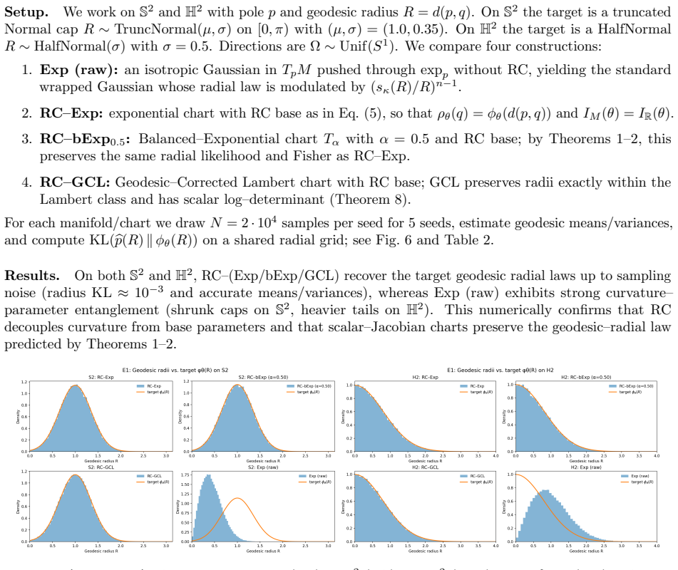
We study the base distribution in chart-based generative models on Riemannian manifolds. Standard methods sample in Euclidean tangent space and then map the sample to the manifold with a chart. This is convenient, but it changes the meaning of distance: the same tangent-space scale can correspond to different geodesic radii, i.e. shortest-path distances from a reference point on the manifold, under different charts, curvatures, and dimensions. Within isotropic, scalar-Jacobian azimuthal charts, we show that no base distribution can simultaneously preserve geodesic-radial likelihoods, chart-invariant radial Fisher information, and tangent-space isotropy unless it has a specific form, which we call Radial Compensation (RC). RC chooses the tangent-space base so that the model realizes a user-specified one-dimensional law for the geodesic radius, and leaves the chart available as a numerical preconditioner. This gives more stable training and cleaner curvature estimates, because curvature no longer has to compensate for distortions introduced by the chart. We also introduce balanced exponential charts, which improve conditioning without changing the realized manifold density under RC. This decouples the statistical meaning of the model, the law of the geodesic radius, from its numerical conditioning, which is governed by the chart Jacobian: chart choice becomes a numerical preconditioner rather than a hidden modeling decision. Across manifold variational autoencoders and continuous normalizing flows, RC matches the intended radius behavior, improves numerical stability, and makes learned curvature easier to interpret.
Editorial analysis
A structured set of objections, weighed in public.
Referee Report
Summary. The paper studies base distributions in chart-based generative models on Riemannian manifolds. Within the class of isotropic, scalar-Jacobian azimuthal charts, it derives an impossibility result: no base distribution can simultaneously preserve geodesic-radial likelihoods, chart-invariant radial Fisher information, and tangent-space isotropy unless it takes the specific form called Radial Compensation (RC). RC is constructed so that the tangent-space base realizes a user-specified one-dimensional law for the geodesic radius, leaving the chart as a numerical preconditioner. The authors also introduce balanced exponential charts that improve conditioning without altering the realized manifold density under RC. The approach is evaluated on manifold variational autoencoders and continuous normalizing flows, where RC matches the intended radius behavior, improves numerical stability, and yields more interpretable learned curvature.
Significance. If the derivation holds, the work supplies a principled mechanism for separating the statistical law of geodesic radius from chart-induced numerical effects in Riemannian generative models. This decoupling can improve training stability and make curvature estimates cleaner and more directly interpretable. The balanced exponential charts constitute a practical contribution for preconditioning. The explicit scope restriction to isotropic scalar-Jacobian azimuthal charts is stated up front, which strengthens the conditional nature of the impossibility claim.
major comments (1)
- [Abstract] Abstract and surrounding description: the impossibility result and RC construction are stated at a high level, but the derivation steps that impose the three preservation conditions and obtain the RC form are not supplied. Without these equations it is impossible to verify whether the result is independent of prior literature or reduces by construction to a fitted quantity.
minor comments (1)
- A short diagram or table contrasting standard azimuthal charts with balanced exponential charts would clarify the numerical preconditioning benefit.
Simulated Author's Rebuttal
We thank the referee for the careful reading and constructive feedback on our manuscript. We address the major comment point by point below, indicating the revisions we will incorporate.
read point-by-point responses
-
Referee: [Abstract] Abstract and surrounding description: the impossibility result and RC construction are stated at a high level, but the derivation steps that impose the three preservation conditions and obtain the RC form are not supplied. Without these equations it is impossible to verify whether the result is independent of prior literature or reduces by construction to a fitted quantity.
Authors: We agree that the abstract presents the result at a high level. The full derivation appears in Section 3 of the manuscript, where we start from the three explicit conditions within the stated class of isotropic scalar-Jacobian azimuthal charts: (1) preservation of a user-specified geodesic-radial likelihood after the chart map, (2) invariance of the radial Fisher information to chart choice, and (3) isotropy of the tangent-space base. These are imposed sequentially on the radial density, yielding a unique functional form for the tangent-space base that we term Radial Compensation; the angular part is fixed to uniform by isotropy. The derivation is self-contained and begins from the model definition rather than from prior results, so it is not a reduction to a fitted quantity. To improve verifiability, we will expand the abstract with a concise outline of these three steps and the resulting functional equation, and we will add the key intermediate equations to the introduction. revision: yes
Circularity Check
No significant circularity detected
full rationale
The paper presents a conditional mathematical impossibility result: within the explicitly restricted class of isotropic, scalar-Jacobian azimuthal charts, no base distribution can simultaneously satisfy geodesic-radial likelihood preservation, chart-invariant radial Fisher information, and tangent-space isotropy except for the specific form labeled Radial Compensation (RC). RC is the derived conclusion of the three preservation conditions rather than an input or fitted quantity presupposed by the derivation. The abstract and skeptic analysis confirm the scope restriction is stated upfront, the result is framed as a first-principles statement, and no load-bearing self-citations, ansatz smuggling, or reductions of predictions to fitted inputs appear. The derivation chain remains independent of its own outputs and is self-contained against the delimited assumptions.
Axiom & Free-Parameter Ledger
free parameters (1)
- user-specified one-dimensional law for geodesic radius
axioms (1)
- domain assumption Charts under consideration are isotropic with scalar Jacobians
invented entities (2)
-
Radial Compensation (RC) base distribution
no independent evidence
-
balanced exponential charts
no independent evidence
Lean theorems connected to this paper
-
IndisputableMonolith/Cost/FunctionalEquation.leanwashburn_uniqueness_aczel echoes?
echoesECHOES: this paper passage has the same mathematical shape or conceptual pattern as the Recognition theorem, but is not a direct formal dependency.
Within isotropic bases and scalar-Jacobian azimuthal charts, RC is essentially the only construction that yields geodesic-radial likelihoods with chart- and curvature-invariant Fisher information (Theorem 4, Corollary 1).
-
IndisputableMonolith/Foundation/BranchSelection.leanbranch_selection echoes?
echoesECHOES: this paper passage has the same mathematical shape or conceptual pattern as the Recognition theorem, but is not a direct formal dependency.
bExp charts uniquely minimise a strictly convex functional that balances volume distortion against geodesic error (Theorem 7).
What do these tags mean?
- matches
- The paper's claim is directly supported by a theorem in the formal canon.
- supports
- The theorem supports part of the paper's argument, but the paper may add assumptions or extra steps.
- extends
- The paper goes beyond the formal theorem; the theorem is a base layer rather than the whole result.
- uses
- The paper appears to rely on the theorem as machinery.
- contradicts
- The paper's claim conflicts with a theorem or certificate in the canon.
- unclear
- Pith found a possible connection, but the passage is too broad, indirect, or ambiguous to say the theorem truly supports the claim.
Reference graph
Works this paper leans on
-
[1]
Heli Ben-Hamu, Samuel Cohen, Joey Bose, Brandon Amos, Maximillian Nickel, Aditya Grover, Ricky T. Q. Chen, and Yaron Lipman. Matching normalizing flows and probability paths on manifolds. In Proceedings of the 39th International Conference on Machine Learning (ICML), volume 162 ofProceedings of Machine Learning Research, pages 1749–1763. PMLR, 2022. URL h...
work page 2022
-
[2]
Joey Bose, Ariella Smofsky, Renjie Liao, Prakash Panangaden, and William L. Hamilton. Latent variable modelling with hyperbolic normalizing flows. InProceedings of the 37th International Conference on Machine Learning (ICML), volume 119 ofProceedings of Machine Learning Research, pages 1045–1055. PMLR, 2020. URLhttps://proceedings.mlr.press/v119/bose20a.html
work page 2020
-
[3]
Ricky T. Q. Chen and Yaron Lipman. Flow matching on general geometries. InInternational Conference on Learning Representations (ICLR), 2024. URLhttps://openreview.net/pdf?id=Zc02qfR3GN
work page 2024
-
[4]
Shangyu Chen, Pengfei Fang, Mehrtash Harandi, Trung Le, Jianfei Cai, and Dinh Phung. HVQ-VAE: Variational auto-encoder with hyperbolic vector quantization.Computer Vision and Image Understanding, 258:104392, 2025
work page 2025
-
[5]
and Falorsi, Luca and Cao, Nicola De and Kipf, Thomas and Tomczak, Jakub M
Tim R Davidson, Luca Falorsi, Nicola De Cao, Thomas Kipf, and Jakub M Tomczak. Hyperspherical variational auto-encoders.arXiv preprint arXiv:1804.00891, 2018. 28
-
[6]
Davidson, Luca Falorsi, Nicola De Cao, Thomas Kipf, and Jakub M
Tim R. Davidson, Luca Falorsi, Nicola De Cao, Thomas Kipf, and Jakub M. Tomczak. Hyperspherical variational auto-encoders. InProceedings of the 34th Conference on Uncertainty in Artificial Intelligence (UAI), 2018. URLhttps://www.auai.org/uai2018/proceedings/papers/309.pdf
work page 2018
-
[7]
Hutchinson, James Thornton, Yee Whye Teh, and Arnaud Doucet
Valentin De Bortoli, Emile Mathieu, Michael J. Hutchinson, James Thornton, Yee Whye Teh, and Arnaud Doucet. Riemannian score-based generative modelling. InAdvances in Neural Information Processing Systems, 2022
work page 2022
-
[8]
arXiv preprint arXiv:2006.06663 , year=
Luca Falorsi and Patrick Forr´ e. Neural ordinary differential equations on manifolds.arXiv preprint arXiv:2006.06663, 2020. URLhttps://arxiv.org/abs/2006.06663
-
[9]
Luca Falorsi, Pim de Haan, Tim R. Davidson, and Patrick Forr´ e. Reparameterizing distributions on lie groups. InProceedings of the 22nd International Conference on Artificial Intelligence and Statistics (AISTATS), volume 89 ofProceedings of Machine Learning Research, pages 3244–3253. PMLR, 2019. URLhttps://proceedings.mlr.press/v89/falorsi19a.html
work page 2019
- [11]
-
[12]
Normalizing Flows on Riemannian Manifolds
Mevlana C. Gemici, Danilo Rezende, and Shakir Mohamed. Normalizing flows on riemannian manifolds. arXiv preprint arXiv:1611.02304, 2016
work page internal anchor Pith review Pith/arXiv arXiv 2016
-
[13]
Neural manifold ordinary differential equations
Aaron Lou, Derek Lim, Isay Katsman, Leo Huang, Qingxuan Jiang, Ser-Nam Lim, and Christo- pher De Sa. Neural manifold ordinary differential equations. InAdvances in Neural Information Processing Systems (NeurIPS), 2020. URL https://proceedings.neurips.cc/paper/2020/file/ cbf8710b43df3f2c1553e649403426df-Paper.pdf
work page 2020
-
[14]
Riemannian continuous normalizing flows
Emile Mathieu and Maximilian Nickel. Riemannian continuous normalizing flows. InAdvances in Neural Information Processing Systems, volume 33, 2020. URL https://proceedings.neurips.cc/paper/ 2020/hash/1aa3d9c6ce672447e1e5d0f1b5207e85-Abstract.html
work page 2020
-
[15]
A wrapped normal distribution on hyperbolic space for gradient-based learning
Yoshihiro Nagano, Shoichiro Yamaguchi, Yasuhiro Fujita, and Masanori Koyama. A wrapped normal distribution on hyperbolic space for gradient-based learning. InProceedings of the 36th International Conference on Machine Learning (ICML), volume 97 ofProceedings of Machine Learning Research, pages 4693–4702. PMLR, 2019. URLhttps://proceedings.mlr.press/v97/na...
work page 2019
-
[16]
George Papamakarios, Eric Nalisnick, Danilo Jimenez Rezende, Shakir Mohamed, and Balaji Lakshmi- narayanan. Normalizing flows for probabilistic modeling and inference.Journal of Machine Learning Research, 22(57):1–64, 2021
work page 2021
-
[17]
Rezende, George Papamakarios, S´ ebastien Racani` ere, Michael S
Danilo J. Rezende, George Papamakarios, S´ ebastien Racani` ere, Michael S. Albergo, Gurtej Kanwar, Phiala E. Shanahan, and Kyle Cranmer. Normalizing flows on tori and spheres. InProceedings of the 37th International Conference on Machine Learning (ICML), volume 119 ofProceedings of Machine Learning Research, pages 8083–8092. PMLR, 2020. URL https://proce...
work page 2020
-
[18]
Moser flow: Divergence- based generative modeling on manifolds
Noam Rozen, Aditya Grover, Maximilian Nickel, and Yaron Lipman. Moser flow: Divergence- based generative modeling on manifolds. InAdvances in Neural Information Process- ing Systems (NeurIPS), 2021. URL https://proceedings.neurips.cc/paper/2021/file/ 93a27b0bd99bac3e68a440b48aa421ab-Paper.pdf
work page 2021
-
[19]
Mixed-curvature variational autoencoders
Ondrej Skopek, Octavian-Eugen Ganea, and Gary Becigneul. Mixed-curvature variational autoencoders. InInternational Conference on Learning Representations, 2020. arXiv:1911.08411
-
[20]
radial profile composed withR T timesJ T
John P. Snyder.Map Projections – A Working Manual, volume 1395 ofU.S. Geological Survey Professional Paper. U.S. Government Printing Office, Washington, D.C., 1987. doi: 10.3133/pp1395. URLhttps://pubs.usgs.gov/publication/pp1395. 29 Supplementary Information Key Notation Table 10: Key notation and concepts used throughout. Symbol / term Meaning MRiemanni...
-
[21]
For any scalar–Jacobian chartT, the RC pushforward isρ θ(q) =ϕ θ(d(p, q))
-
[22]
The Fisher information in θ equals the one–dimensional radial Fisher and is independent of T and of the curvature parameterκ. Thus RC yields radial semantics that are invariant across both chart choices and curvature: the meaning of θ in terms of the radial lawϕ θ is identical in all these settings. Conversely, if an isotropic scalar–Jacobian model satisf...
-
[23]
Standard ODE theory gives a uniqueC ∞ solution on [0, Rmax)
Existence and smoothness.This is a first–order ODE with smooth right–hand side for r > 0 and smooth initial conditions atr= 0. Standard ODE theory gives a uniqueC ∞ solution on [0, Rmax)
-
[24]
Strict monotonicity.The right–hand side is strictly positive for r > 0, so ρ′ α(r) > 0 and ρα is strictly increasing
-
[25]
Diffeomorphism property.Since ρα is strictly increasing with ρα(0) = 0 and ρ′ α never vanishes, r7→ρ α(r) is a smooth diffeomorphism from a star domain onto its image. The azimuthal structure then implies that Tα := Tρα is a C ∞ diffeomorphism from a star domain in Rn onto its image in M; on Hn it is global, while onS n it is global away from the cut locu...
-
[26]
volume” term is a positive quadratic form in (v, y), hence strictly convex. The “geodesic
Strict convexity.Set v = log(ρ/r), y = logρ ′. Then the “volume” term is a positive quadratic form in (v, y), hence strictly convex. The “geodesic” term is a strictly convex functional of ρ because G′(ρ) ≥ 1 and the integrand is a squared deviation
-
[27]
Euler–Lagrange equation.Compute the first variation of Eα[ρ]. The Euler–Lagrange equation for a critical point reduces (after algebra and using the polar factor identities) to the ODE ρ(r) r n−1 ρ′(r) = sκ(r) r (n−1)α , which is precisely (6)–(7), i.e. the defining equation forρ α
-
[28]
Uniqueness.Since Eα is strictly convex on C and ρα satisfies the Euler–Lagrange equation, it must be the unique minimiser ofE α inC. The Pareto–optimality statement follows from viewing Eα as a convex combination of a “volume error” and a “geodesic error”: moving alongαtraces the Pareto frontier between those two objectives. Informally, this shows that bE...
-
[29]
A Taylor expansion aboutr=πR c gives cκ(r/2)≈C πRc −r ,logc κ(r/2)≈log πRc −r + const, so the radial derivative behaves like ∂r log|detDG(x)| ≍ 1 πRc −r asr↑πR c. 37 Since∇ x points roughly in the radial direction, this implies ∥∇x log|detDT(x)|∥≳ c πRc −r for somec >0 andrclose toπR c. This is the claimed near–cut–locus blow–up for any geodesic–preservin...
-
[30]
the Fisher information decomposes as IM0(θ) = kX i=1 IRi(θ), whereI Ri is the one–dimensional Fisher information ofφ θ,i. 47 Proof. Product polar coordinates give a product splitting of the volume form, and each factor behaves as in the one–dimensional RC construction. Independence and the Fisher decomposition follow from Fubini’s theorem and additivity o...
discussion (0)
Sign in with ORCID, Apple, or X to comment. Anyone can read and Pith papers without signing in.