Continuous-time Online Learning via Mean-Field Neural Networks: Regret Analysis in Diffusion Environments

Bingyan Han; Erhan Bayraktar; Ziqing Zhang

arxiv: 2604.10958 · v1 · submitted 2026-04-13 · 💻 cs.LG · cs.AI· math.OC

Continuous-time Online Learning via Mean-Field Neural Networks: Regret Analysis in Diffusion Environments

Erhan Bayraktar , Bingyan Han , Ziqing Zhang This is my paper

Pith reviewed 2026-05-10 16:07 UTC · model grok-4.3

classification 💻 cs.LG cs.AImath.OC

keywords continuous-time online learningmean-field neural networksregret boundsdiffusion processesWasserstein gradient flowdisplacement convexityPolyak-Lojasiewicz conditionpropagation of chaos

0 comments

The pith

Mean-field neural networks achieve constant static regret for continuous-time online learning from diffusion data under displacement convexity, and explicit linear regret otherwise.

A machine-rendered reading of the paper's core claim, the machinery that carries it, and where it could break.

This paper studies continuous-time online learning in which data arrives from an unknown diffusion process and the learner deploys a two-layer neural network whose parameters evolve continuously and non-anticipatively. The mean-field limit of the dynamics is shown to be a stochastic Wasserstein gradient flow adapted to the data filtration. Under displacement convexity the static regret stays bounded by a constant; in the general non-convex setting the regret grows linearly with explicit dependence on data variation, entropic exploration, and quadratic regularization. The same bounds hold for finite-particle approximations through uniform-in-time propagation of chaos. These guarantees matter because they supply theoretical control for neural-network training on streaming data whose statistics change continuously according to a diffusion law.

Core claim

The mean-field limit of non-anticipative parameter updates driven by diffusion data corresponds to a stochastic Wasserstein gradient flow adapted to the filtration; under displacement convexity this flow yields constant static regret, while in the non-convex case explicit linear regret bounds are obtained that isolate the effects of data variation, entropic exploration, and quadratic regularization. The analysis relies on the logarithmic Sobolev inequality, the Polyak-Lojasiewicz condition, Malliavin calculus, and uniform propagation of chaos to extend the bounds from the mean-field limit to finite-particle systems.

What carries the argument

the stochastic Wasserstein gradient flow adapted to the data filtration, which evolves the empirical measure of network parameters and permits regret control via functional inequalities

If this is right

Constant regret independent of time horizon is attained whenever the loss is displacement convex.
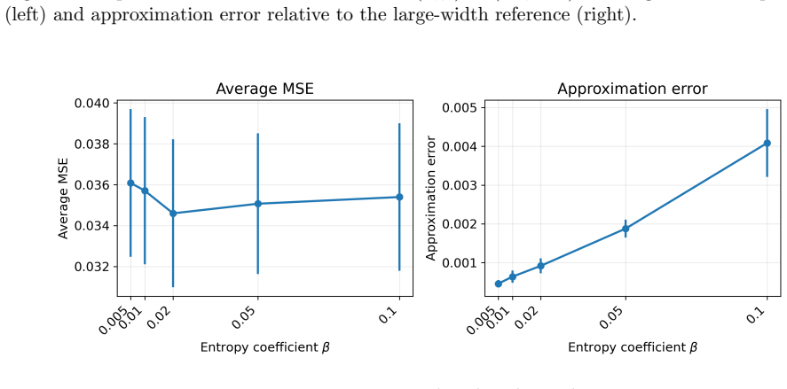
In non-convex regimes the linear growth rate is explicitly modulated by the size of data variation, the entropic exploration coefficient, and the strength of quadratic regularization.
Finite-width networks inherit the same regret guarantees once uniform-in-time propagation of chaos is established.
The results apply directly to any data stream whose law is a diffusion with fixed coefficients.

Where Pith is reading between the lines

These are editorial extensions of the paper, not claims the author makes directly.

The same functional-inequality approach might extend regret analysis to data generated by other continuous-time processes such as jump diffusions, provided analogous Sobolev-type inequalities hold.
Discretizing the mean-field flow could yield practical online algorithms whose performance tracks the continuous-time bounds for streaming neural-network training.
The explicit dependence on regularization and width parameters supplies a guide for tuning finite networks on real diffusion-like data streams.

Load-bearing premise

The data must be generated by a diffusion process whose coefficients are unknown but fixed, and the loss must satisfy either displacement convexity or the Polyak-Lojasiewicz condition.

What would settle it

Empirical observation that regret grows faster than linear when diffusion coefficients vary arbitrarily or when the loss violates displacement convexity and the Polyak-Lojasiewicz condition would disprove the stated bounds.

Figures

Figures reproduced from arXiv: 2604.10958 by Bingyan Han, Erhan Bayraktar, Ziqing Zhang.

**Figure 2.** Figure 2: Unregularized regret dynamics. The panel layout and parameter variations are identical [PITH_FULL_IMAGE:figures/full_fig_p028_2.png] view at source ↗

**Figure 3.** Figure 3: Impact of network width N at fixed (λ, β) = (0.1, 0.02). Average out-of-sample MSE (left) and approximation error relative to the large-width reference (right) [PITH_FULL_IMAGE:figures/full_fig_p029_3.png] view at source ↗

**Figure 4.** Figure 4: Impact of entropy coefficient β at fixed (N, λ) = (80, 0.1). Average out-of-sample MSE (left) and approximation error relative to the large-width reference (right). Figures 3, 4, and 5 evaluate out-of-sample performance across various parameters. All panels display sample means and 95% confidence intervals computed across repeated trials. The left panels report the average out-of-sample MSE defined in (6.2… view at source ↗

**Figure 5.** Figure 5: Impact of L 2 regularization parameter λ at fixed (N, β) = (80, 0.02). Average out-ofsample MSE (left) and approximation error relative to the large-width reference (right). approximation error relative to the estimated instantaneous optimal measure ˆµtk , given by 1 K X K k=1 Z σ(Xtest tk , θ) ˆρ N tk (dθ) − Z σ(Xtest tk , θ) ˆµtk (dθ) 2 , where ˆµtk can also be obtained by training a large network on … view at source ↗

read the original abstract

We study continuous-time online learning where data are generated by a diffusion process with unknown coefficients. The learner employs a two-layer neural network, continuously updating its parameters in a non-anticipative manner. The mean-field limit of the learning dynamics corresponds to a stochastic Wasserstein gradient flow adapted to the data filtration. We establish regret bounds for both the mean-field limit and finite-particle system. Our analysis leverages the logarithmic Sobolev inequality, Polyak-Lojasiewicz condition, Malliavin calculus, and uniform-in-time propagation of chaos. Under displacement convexity, we obtain a constant static regret bound. In the general non-convex setting, we derive explicit linear regret bounds characterizing the effects of data variation, entropic exploration, and quadratic regularization. Finally, our simulations demonstrate the outperformance of the online approach and the impact of network width and regularization parameters.

Editorial analysis

A structured set of objections, weighed in public.

Desk editor's note, referee report, simulated authors' rebuttal, and a circularity audit. Tearing a paper down is the easy half of reading it; the pith above is the substance, this is the friction.

Desk Editor's Note private letter to a colleague

Regret bounds for mean-field NN online learning in diffusions, but they rest on standing assumptions about loss convexity and fixed diffusion coefficients that are not shown to hold for two-layer networks.

read the letter

This paper gives explicit regret bounds for continuous-time online learning with two-layer neural networks in a mean-field limit when data is generated by a diffusion. Under displacement convexity they get constant static regret; otherwise they get linear regret with explicit factors for data variation, entropic exploration, and quadratic regularization. They also carry the bounds to the finite-particle system. The setup uses non-anticipative updates and a stochastic Wasserstein gradient flow adapted to the data filtration, then applies logarithmic Sobolev inequalities, the Polyak-Lojasiewicz condition, Malliavin calculus, and uniform-in-time propagation of chaos. That combination for this continuous-time diffusion setting looks new compared with prior discrete-time or non-diffusion work, and the explicit parameter dependence is a plus. The non-anticipative handling and the mean-field to particle extension are handled with care. The soft spot is that displacement convexity or the PL inequality is treated as a standing assumption on the population loss under the diffusion measure rather than something derived for the two-layer network loss. The diffusion coefficients are also assumed time-independent. If either fails, the Gronwall estimates and the step from flow to regret do not close. The abstract mentions simulations showing outperformance and the effect of width and regularization, but without details it is unclear how strongly they back the theory. This is for readers working on theoretical online learning, mean-field limits, or stochastic control who need regret guarantees in continuous-time diffusion environments. It is worth a serious referee to check whether the assumptions can be verified or relaxed for actual neural-network losses and to see the full derivations.

Referee Report

2 major / 2 minor

Summary. The manuscript studies continuous-time online learning with data generated by a diffusion process with unknown but fixed coefficients. A two-layer neural network is updated continuously in a non-anticipative manner; its mean-field limit is a stochastic Wasserstein gradient flow. Regret bounds are derived for both the mean-field limit and the finite-particle system by combining the logarithmic Sobolev inequality, the Polyak-Łojasiewicz condition, Malliavin calculus, and uniform-in-time propagation of chaos. Under displacement convexity a constant static regret bound is obtained; in the general non-convex case explicit linear regret bounds are given that isolate the effects of data variation, entropic exploration, and quadratic regularization. Simulations illustrate the advantage of the online approach and the role of network width and regularization.

Significance. If the stated assumptions hold, the work supplies the first explicit regret guarantees for mean-field neural-network dynamics in a continuous-time diffusive environment, cleanly separating the contributions of convexity, data variation, and regularization. The technical toolkit (Malliavin calculus plus propagation of chaos) is appropriate and the distinction between the displacement-convex and PL regimes is useful. The results remain conditional on strong structural hypotheses whose validity for two-layer networks under diffusion measures is not established in the manuscript, which tempers the immediate scope of the contribution.

major comments (2)

[Abstract] Abstract and the statement of the main theorems: the constant-regret claim under displacement convexity and the linear-regret claim in the non-convex case both rest on the standing assumption that the population loss satisfies displacement convexity or the Polyak-Łojasiewicz inequality with respect to the diffusion measure. The manuscript does not verify that the two-layer neural-network loss obeys either condition; if the assumption fails, the Gronwall-type estimates used to convert the continuous-time flow into a regret bound no longer close. This is load-bearing for both headline results.
[Introduction / Model section] The analysis throughout invokes that the data-generating diffusion has time-independent coefficients. No argument is given that the regret bounds remain valid (or can be modified) when the diffusion coefficients vary with time in a non-diffusive manner, yet the title and abstract present the setting as general diffusion environments.

minor comments (2)

[Main theorems] The dependence of the linear regret bound on the quadratic regularization strength and network width should be stated explicitly in the theorem statements rather than only in the simulation discussion.
[Preliminaries] Notation for the stochastic Wasserstein gradient flow and the filtration-adapted processes is introduced without a consolidated table of symbols; this makes the propagation-of-chaos argument harder to follow.

Simulated Author's Rebuttal

2 responses · 1 unresolved

We appreciate the referee's detailed feedback on our manuscript. The comments raise important points about the assumptions underlying our regret bounds and the scope of the diffusion setting. We address each major comment below and indicate the revisions we plan to make.

read point-by-point responses

Referee: [Abstract] Abstract and the statement of the main theorems: the constant-regret claim under displacement convexity and the linear-regret claim in the non-convex case both rest on the standing assumption that the population loss satisfies displacement convexity or the Polyak-Łojasiewicz inequality with respect to the diffusion measure. The manuscript does not verify that the two-layer neural-network loss obeys either condition; if the assumption fails, the Gronwall-type estimates used to convert the continuous-time flow into a regret bound no longer close. This is load-bearing for both headline results.

Authors: We thank the referee for highlighting this point. The main theorems are indeed stated under the assumption that the population loss satisfies either displacement convexity or the Polyak-Łojasiewicz (PL) inequality with respect to the underlying diffusion measure. This is explicitly noted in the statements of the main theorems. Verifying these structural properties for the specific two-layer neural network loss function under a general diffusion measure is a non-trivial task that depends on the choice of activation functions, network architecture, and the specific form of the loss; it lies beyond the scope of the current work, which focuses on deriving regret bounds conditional on these properties. We will revise the abstract and the introduction to more clearly state that the results hold under these assumptions, and add a discussion regarding the plausibility of these conditions for neural network losses in diffusive settings. revision: yes
Referee: [Introduction / Model section] The analysis throughout invokes that the data-generating diffusion has time-independent coefficients. No argument is given that the regret bounds remain valid (or can be modified) when the diffusion coefficients vary with time in a non-diffusive manner, yet the title and abstract present the setting as general diffusion environments.

Authors: The problem formulation in Section 2 explicitly assumes a diffusion process with time-independent coefficients, which enables the uniform-in-time propagation of chaos and the application of Malliavin calculus in the analysis. The title and abstract refer to 'diffusion environments' in this context, but we agree that greater precision is warranted to avoid misinterpretation. We will revise the abstract to specify 'time-homogeneous diffusion processes with unknown coefficients' and add a remark in the introduction clarifying the time-independence assumption, noting that extensions to time-varying coefficients are left for future research. revision: yes

standing simulated objections not resolved

The verification that the two-layer neural-network loss satisfies displacement convexity or the Polyak-Łojasiewicz inequality with respect to the diffusion measure.

Circularity Check

0 steps flagged

Regret bounds derived from external inequalities and stated assumptions with no reduction to inputs by construction

full rationale

The derivation applies standard tools (logarithmic Sobolev, PL inequality, Malliavin calculus, uniform propagation of chaos) to the stochastic Wasserstein gradient flow under explicitly stated standing assumptions on the diffusion coefficients and on the loss (displacement convexity or PL). These assumptions are not derived from the two-layer NN model itself within the paper, nor are any regret quantities fitted to data and then relabeled as predictions. No self-citation chain is load-bearing for the central bounds, and no equation reduces to a prior equation by renaming or self-definition. The analysis is therefore self-contained against external analytic benchmarks.

Axiom & Free-Parameter Ledger

2 free parameters · 2 axioms · 0 invented entities

The central claims rest on standard analytic inequalities (logarithmic Sobolev, Polyak-Lojasiewicz) applied to a new stochastic Wasserstein gradient flow; no new entities are postulated and the only free parameters appear to be network width and regularization strength, which are varied in simulations rather than fitted to derive the bounds.

free parameters (2)

network width
Mentioned as impacting performance in simulations; treated as a tunable parameter rather than derived.
quadratic regularization strength
Appears in the linear regret bound expression and is varied in experiments.

axioms (2)

domain assumption Data generated by a diffusion process with unknown coefficients
Stated in the opening sentence of the abstract as the environment for the online learning problem.
domain assumption Loss satisfies displacement convexity or Polyak-Lojasiewicz condition
Invoked to obtain constant versus linear regret bounds.

pith-pipeline@v0.9.0 · 5454 in / 1570 out tokens · 58964 ms · 2026-05-10T16:07:30.800220+00:00 · methodology

discussion (0)

Reference graph

Works this paper leans on

10 extracted references · 10 canonical work pages

[1]

Existence, uniqueness, and the uniformL ∞ bound.We use the fixed-point argument in Proposition 4.3 of Monmarch´ e et al. (2024). FixT∈(0,∞), and define X:=C [0, T];L 1(Rd)∩ P(R d) equipped with the uniform metric d(µ, ν) := sup t∈[0,T] ∥µt −ν t∥L1, forµ, ν∈ X. Ifµ∈ X, thenµ t is a probability measure and has a density function, still denoted byµ t. Clearl...

work page 2024
[2]

This gives a differential inequality for Z Rd Vk(θ)ρ t(dθ), from which we obtain the uniform bound on thek-th moment

Uniform moment bound.We can calculate the expectation of the Lyapunov function Vk(θ) := (1 +|θ| 2)k/2. This gives a differential inequality for Z Rd Vk(θ)ρ t(dθ), from which we obtain the uniform bound on thek-th moment. The details are omitted here for simplicity

work page
[3]

Define bε(µt, Zt, θ) =λθ+ 2 ⟨µt, σε(Xt,·)⟩ −Y t ∇σε(Xt, θ)

Stability with respect to the approximation.Letσ ε =σ∗η ε be the mollified function. Define bε(µt, Zt, θ) =λθ+ 2 ⟨µt, σε(Xt,·)⟩ −Y t ∇σε(Xt, θ). Thenb ε satisfies the same conditions asbin Monmarch´ e et al. (2024, Proposition A.1). It follows that ∥ρt −ρ ε t ∥L1 ≤e C′t∥ρ0 −ρ ε 0∥L1 +C ′√ tsup s∈[0,t] ∥b(ρs, Zs, θ)−b ε(ρε s, Zs, θ)∥L∞, whereρ ε is the uni...

work page 2024
[4]

Supposeφ t =φ 1,t +φ 2,t with boundedφ 1,t andL 2-Lipschitzφ 2,t for allt∈[0, T], then ∥∇ut∥L∞ ≤Ce −ct∥∇u0∥L∞ +C Z t 0 e−cs ∥φ1,t−s∥L∞ √ s∧1 +L 2 ds, t∈[0, T],(A.5) whereC,c >0and depend only onκ ˜b andβ

work page
[5]

Proof of Lemma A.1.A direct calculation shows thatu t satisfies ∂tut =β∆u t −β|∇u t|2 + ˜bt · ∇ut +φ t =β∆u t + inf α β|α|2 −2βα· ∇u t + ˜bt · ∇ut +φ t

If additionally,∇φ t ∈L ∞ for allt∈[0, T], then ∥D2ut∥L∞ ≤ C′e−c′t √ t∧1 ∥∇u0∥L∞ + Z t 0 C′e−c′v √ v∧1 ∥∇φt−v∥L∞ +∥∇ ˜bt−v · ∇ut−v∥L∞ dv, (A.6) for allt∈[0, T], whereC ′,c ′ >0and depend only onκ ˜b,β,∥∇u 0∥L∞, andsup t∈[0,T] ∥φt∥L∞. Proof of Lemma A.1.A direct calculation shows thatu t satisfies ∂tut =β∆u t −β|∇u t|2 + ˜bt · ∇ut +φ t =β∆u t + inf α β|α|2...

work page 2016
[6]

Denoteu i(t) :=⟨ρ ∗ i , σ(Xt,·)⟩,i= 1,2

Note that Hi(θ) := λ 2β |θ|2 + 2 βT Z T 0 (⟨ρ∗ i , σ(Xt,·)⟩ −Y t)σ(X t, θ)dt=−logρ ∗ i (θ)−logA i, i= 1,2, whereA i is the normalization constant inρ ∗ i . Denoteu i(t) :=⟨ρ ∗ i , σ(Xt,·)⟩,i= 1,2. Then the first form ofH i implies that H1(θ)−H 2(θ) = 2 βT Z T 0 (u1(t)−u 2(t))σ(Xt, θ)dt. Multiplying both sides byρ ∗ 1 −ρ ∗ 2 and integrating overθ, Z (ρ∗ 1(...

work page 2008
[7]

|(Fx(ρt, Zt)−F x(µ∗ t , Zt))⊤b1| ≤2|b 1||⟨ρt, σ(Xt,·)⟩⟨ρ t, σx(Xt,·)⟩ − ⟨µ ∗ t , σ(Xt,·)⟩⟨µ ∗ t , σx(Xt,·)⟩| + 2Cz|b1||⟨ρt, σx(Xt,·)⟩ − ⟨µ ∗ t , σx(Xt,·)⟩|

Theb 1 term inA[F](ρ t, Zt)− A[F](µ ∗ t , Zt). |(Fx(ρt, Zt)−F x(µ∗ t , Zt))⊤b1| ≤2|b 1||⟨ρt, σ(Xt,·)⟩⟨ρ t, σx(Xt,·)⟩ − ⟨µ ∗ t , σ(Xt,·)⟩⟨µ ∗ t , σx(Xt,·)⟩| + 2Cz|b1||⟨ρt, σx(Xt,·)⟩ − ⟨µ ∗ t , σx(Xt,·)⟩|. Thanks to Assumption 3.1 and the strong duality of Wasserstein distance of order 1, we have |⟨ρt, σ(Xt,·)⟩⟨ρ t, σx(Xt,·)⟩ − ⟨µ ∗ t , σ(Xt,·)⟩⟨µ ∗ t , σx(...

work page
[8]

We use|σ θ| ≤C 1 to obtain |(Fy(ρt, Zt)−F y(µ∗ t , Zt))b2| ≤2|b 2| |⟨ρt, σ(Xt,·)⟩ − ⟨µ ∗ t , σ(Xt,·)⟩| ≤2|b 2|C1W1(ρt, µ∗ t )

Theb 2 term inA[F](ρ t, Zt)− A[F](µ ∗ t , Zt). We use|σ θ| ≤C 1 to obtain |(Fy(ρt, Zt)−F y(µ∗ t , Zt))b2| ≤2|b 2| |⟨ρt, σ(Xt,·)⟩ − ⟨µ ∗ t , σ(Xt,·)⟩| ≤2|b 2|C1W1(ρt, µ∗ t )

work page
[9]

We need to bound 1 2tr[(Fxx(ρt, Zt)−F xx(µ∗ t , Zt))Σ1Σ⊤ 1 ]

The Σ 1Σ⊤ 1 term inA[F](ρ t, Zt)− A[F](µ ∗ t , Zt). We need to bound 1 2tr[(Fxx(ρt, Zt)−F xx(µ∗ t , Zt))Σ1Σ⊤ 1 ]. It suffices to bound the norm of the difference of the Hessian matrices. |Fxx(ρt, Zt)−F xx(µ∗ t , Zt)| ≤2|⟨ρ t, σ⟩⟨ρt, σxx⟩ − ⟨µ∗ t , σ⟩⟨µ∗ t , σxx⟩| + 2|⟨ρt, σx⟩⟨ρt, σx⟩⊤ − ⟨µ∗ t , σx⟩⟨µ∗ t , σx⟩⊤| + 2|Yt||⟨ρt, σxx⟩ − ⟨µ∗ t , σxx⟩|. We handle...

work page
[10]

The Σ 1Σ⊤ 2 term inA[F](ρ t, Zt)− A[F](µ ∗ t , Zt). We have |tr[(Fyx(ρt, Zt)−F yx(µ∗ t , Zt))Σ1Σ⊤ 2 ]| ≤ |Σ1Σ⊤ 2 ||Fyx(ρt, Zt)−F yx(µ∗ t , Zt)| = 2|Σ1Σ⊤ 2 ||⟨ρt, σx⟩ − ⟨µ∗ t , σx⟩| ≤2|Σ 1Σ⊤ 2 |C2W1(ρt, µ∗ t )≤C 2(|Σ1Σ⊤ 1 |+|Σ 2Σ⊤ 2 |)W1(ρt, µ∗ t ). In the last inequality, we used|Σ 1Σ⊤ 2 | ≤ 1 2(|Σ1Σ⊤ 1 |+|Σ 2Σ⊤ 2 |). 51 For notational simplicity, we defi...

work page 2000

[1] [1]

Existence, uniqueness, and the uniformL ∞ bound.We use the fixed-point argument in Proposition 4.3 of Monmarch´ e et al. (2024). FixT∈(0,∞), and define X:=C [0, T];L 1(Rd)∩ P(R d) equipped with the uniform metric d(µ, ν) := sup t∈[0,T] ∥µt −ν t∥L1, forµ, ν∈ X. Ifµ∈ X, thenµ t is a probability measure and has a density function, still denoted byµ t. Clearl...

work page 2024

[2] [2]

This gives a differential inequality for Z Rd Vk(θ)ρ t(dθ), from which we obtain the uniform bound on thek-th moment

Uniform moment bound.We can calculate the expectation of the Lyapunov function Vk(θ) := (1 +|θ| 2)k/2. This gives a differential inequality for Z Rd Vk(θ)ρ t(dθ), from which we obtain the uniform bound on thek-th moment. The details are omitted here for simplicity

work page

[3] [3]

Define bε(µt, Zt, θ) =λθ+ 2 ⟨µt, σε(Xt,·)⟩ −Y t ∇σε(Xt, θ)

Stability with respect to the approximation.Letσ ε =σ∗η ε be the mollified function. Define bε(µt, Zt, θ) =λθ+ 2 ⟨µt, σε(Xt,·)⟩ −Y t ∇σε(Xt, θ). Thenb ε satisfies the same conditions asbin Monmarch´ e et al. (2024, Proposition A.1). It follows that ∥ρt −ρ ε t ∥L1 ≤e C′t∥ρ0 −ρ ε 0∥L1 +C ′√ tsup s∈[0,t] ∥b(ρs, Zs, θ)−b ε(ρε s, Zs, θ)∥L∞, whereρ ε is the uni...

work page 2024

[4] [4]

Supposeφ t =φ 1,t +φ 2,t with boundedφ 1,t andL 2-Lipschitzφ 2,t for allt∈[0, T], then ∥∇ut∥L∞ ≤Ce −ct∥∇u0∥L∞ +C Z t 0 e−cs ∥φ1,t−s∥L∞ √ s∧1 +L 2 ds, t∈[0, T],(A.5) whereC,c >0and depend only onκ ˜b andβ

work page

[5] [5]

Proof of Lemma A.1.A direct calculation shows thatu t satisfies ∂tut =β∆u t −β|∇u t|2 + ˜bt · ∇ut +φ t =β∆u t + inf α β|α|2 −2βα· ∇u t + ˜bt · ∇ut +φ t

If additionally,∇φ t ∈L ∞ for allt∈[0, T], then ∥D2ut∥L∞ ≤ C′e−c′t √ t∧1 ∥∇u0∥L∞ + Z t 0 C′e−c′v √ v∧1 ∥∇φt−v∥L∞ +∥∇ ˜bt−v · ∇ut−v∥L∞ dv, (A.6) for allt∈[0, T], whereC ′,c ′ >0and depend only onκ ˜b,β,∥∇u 0∥L∞, andsup t∈[0,T] ∥φt∥L∞. Proof of Lemma A.1.A direct calculation shows thatu t satisfies ∂tut =β∆u t −β|∇u t|2 + ˜bt · ∇ut +φ t =β∆u t + inf α β|α|2...

work page 2016

[6] [6]

Denoteu i(t) :=⟨ρ ∗ i , σ(Xt,·)⟩,i= 1,2

Note that Hi(θ) := λ 2β |θ|2 + 2 βT Z T 0 (⟨ρ∗ i , σ(Xt,·)⟩ −Y t)σ(X t, θ)dt=−logρ ∗ i (θ)−logA i, i= 1,2, whereA i is the normalization constant inρ ∗ i . Denoteu i(t) :=⟨ρ ∗ i , σ(Xt,·)⟩,i= 1,2. Then the first form ofH i implies that H1(θ)−H 2(θ) = 2 βT Z T 0 (u1(t)−u 2(t))σ(Xt, θ)dt. Multiplying both sides byρ ∗ 1 −ρ ∗ 2 and integrating overθ, Z (ρ∗ 1(...

work page 2008

[7] [7]

|(Fx(ρt, Zt)−F x(µ∗ t , Zt))⊤b1| ≤2|b 1||⟨ρt, σ(Xt,·)⟩⟨ρ t, σx(Xt,·)⟩ − ⟨µ ∗ t , σ(Xt,·)⟩⟨µ ∗ t , σx(Xt,·)⟩| + 2Cz|b1||⟨ρt, σx(Xt,·)⟩ − ⟨µ ∗ t , σx(Xt,·)⟩|

Theb 1 term inA[F](ρ t, Zt)− A[F](µ ∗ t , Zt). |(Fx(ρt, Zt)−F x(µ∗ t , Zt))⊤b1| ≤2|b 1||⟨ρt, σ(Xt,·)⟩⟨ρ t, σx(Xt,·)⟩ − ⟨µ ∗ t , σ(Xt,·)⟩⟨µ ∗ t , σx(Xt,·)⟩| + 2Cz|b1||⟨ρt, σx(Xt,·)⟩ − ⟨µ ∗ t , σx(Xt,·)⟩|. Thanks to Assumption 3.1 and the strong duality of Wasserstein distance of order 1, we have |⟨ρt, σ(Xt,·)⟩⟨ρ t, σx(Xt,·)⟩ − ⟨µ ∗ t , σ(Xt,·)⟩⟨µ ∗ t , σx(...

work page

[8] [8]

We use|σ θ| ≤C 1 to obtain |(Fy(ρt, Zt)−F y(µ∗ t , Zt))b2| ≤2|b 2| |⟨ρt, σ(Xt,·)⟩ − ⟨µ ∗ t , σ(Xt,·)⟩| ≤2|b 2|C1W1(ρt, µ∗ t )

Theb 2 term inA[F](ρ t, Zt)− A[F](µ ∗ t , Zt). We use|σ θ| ≤C 1 to obtain |(Fy(ρt, Zt)−F y(µ∗ t , Zt))b2| ≤2|b 2| |⟨ρt, σ(Xt,·)⟩ − ⟨µ ∗ t , σ(Xt,·)⟩| ≤2|b 2|C1W1(ρt, µ∗ t )

work page

[9] [9]

We need to bound 1 2tr[(Fxx(ρt, Zt)−F xx(µ∗ t , Zt))Σ1Σ⊤ 1 ]

The Σ 1Σ⊤ 1 term inA[F](ρ t, Zt)− A[F](µ ∗ t , Zt). We need to bound 1 2tr[(Fxx(ρt, Zt)−F xx(µ∗ t , Zt))Σ1Σ⊤ 1 ]. It suffices to bound the norm of the difference of the Hessian matrices. |Fxx(ρt, Zt)−F xx(µ∗ t , Zt)| ≤2|⟨ρ t, σ⟩⟨ρt, σxx⟩ − ⟨µ∗ t , σ⟩⟨µ∗ t , σxx⟩| + 2|⟨ρt, σx⟩⟨ρt, σx⟩⊤ − ⟨µ∗ t , σx⟩⟨µ∗ t , σx⟩⊤| + 2|Yt||⟨ρt, σxx⟩ − ⟨µ∗ t , σxx⟩|. We handle...

work page

[10] [10]

The Σ 1Σ⊤ 2 term inA[F](ρ t, Zt)− A[F](µ ∗ t , Zt). We have |tr[(Fyx(ρt, Zt)−F yx(µ∗ t , Zt))Σ1Σ⊤ 2 ]| ≤ |Σ1Σ⊤ 2 ||Fyx(ρt, Zt)−F yx(µ∗ t , Zt)| = 2|Σ1Σ⊤ 2 ||⟨ρt, σx⟩ − ⟨µ∗ t , σx⟩| ≤2|Σ 1Σ⊤ 2 |C2W1(ρt, µ∗ t )≤C 2(|Σ1Σ⊤ 1 |+|Σ 2Σ⊤ 2 |)W1(ρt, µ∗ t ). In the last inequality, we used|Σ 1Σ⊤ 2 | ≤ 1 2(|Σ1Σ⊤ 1 |+|Σ 2Σ⊤ 2 |). 51 For notational simplicity, we defi...

work page 2000