Neural Spectral Element Methods for stiff multiphysics PDEs with electrochemical transport benchmarks
Pith reviewed 2026-06-28 13:30 UTC · model grok-4.3
The pith
The Neural Spectral Element Method solves stiff electrochemical PDEs to 10^-4--10^-7 error using two orders of magnitude fewer collocation points than PINNs.
A machine-rendered reading of the paper's core claim, the machinery that carries it, and where it could break.
Core claim
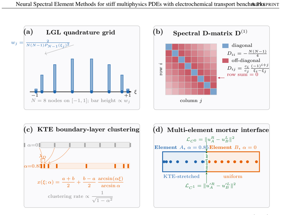
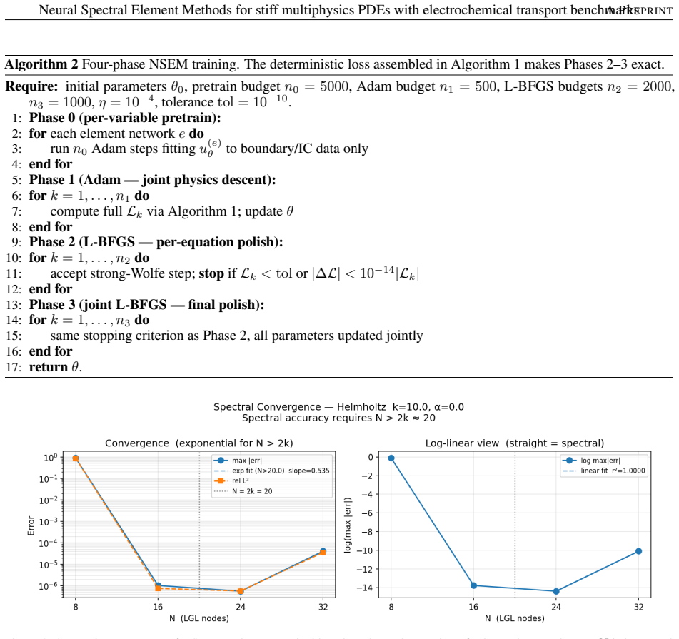
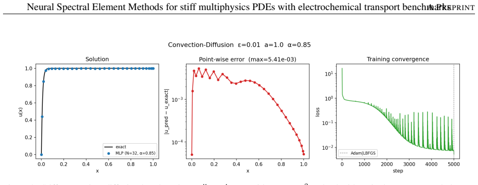
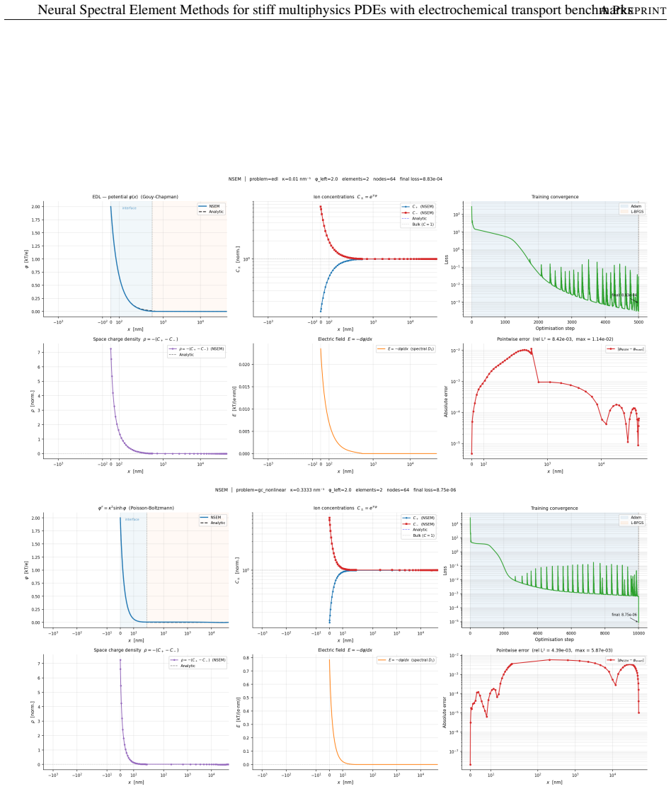
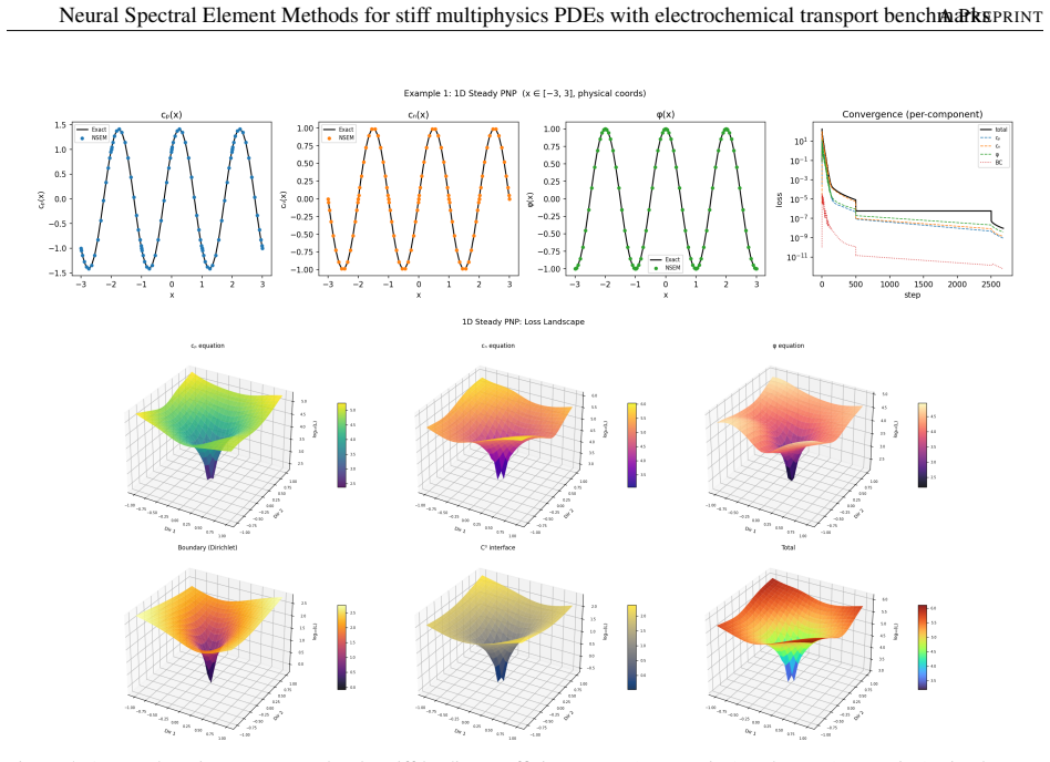
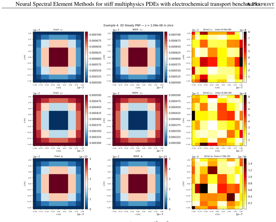
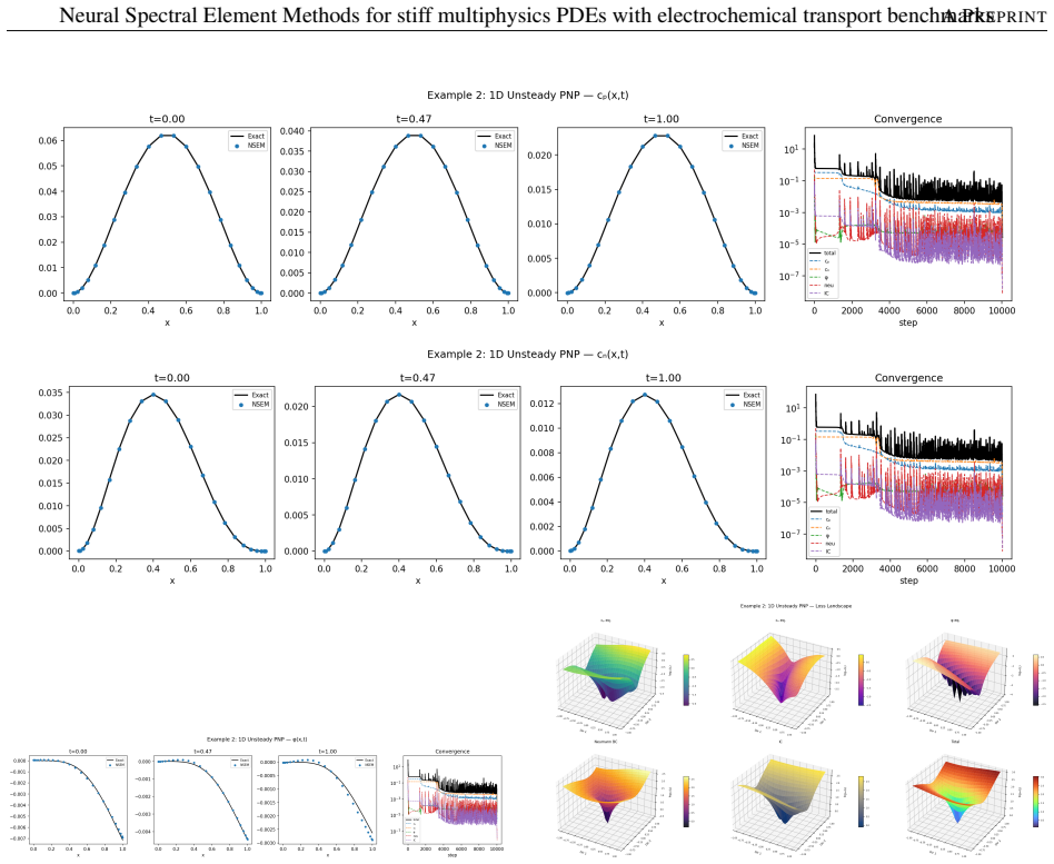
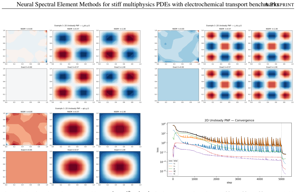
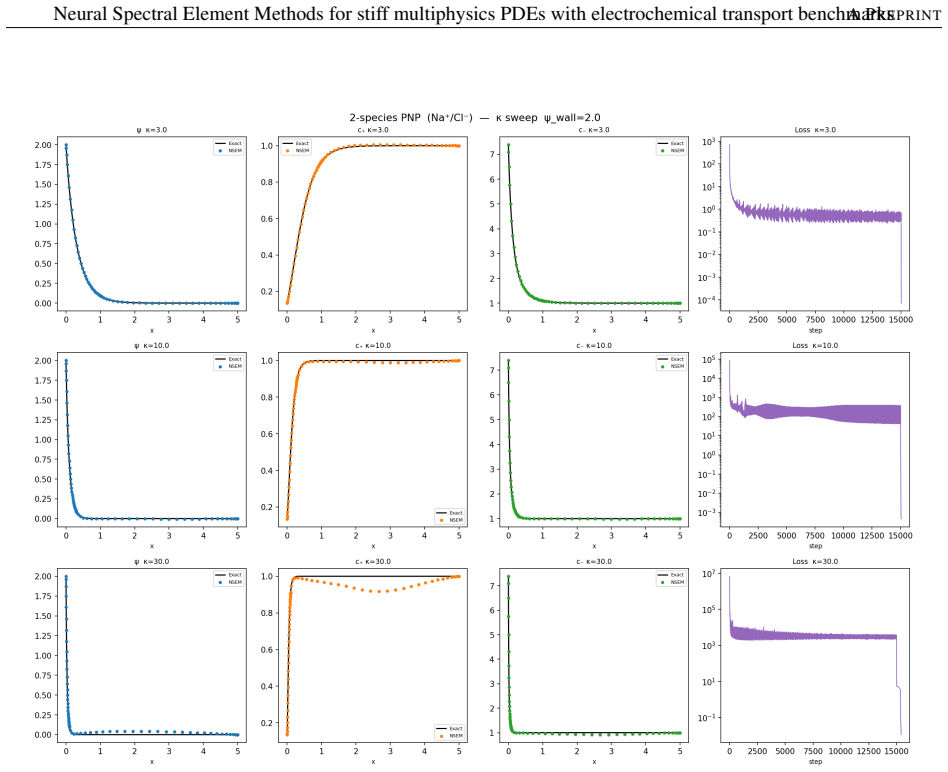
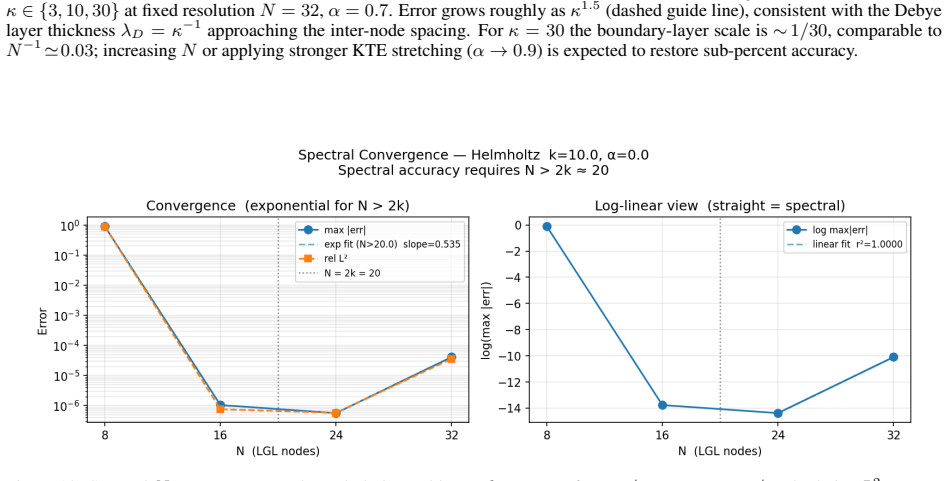
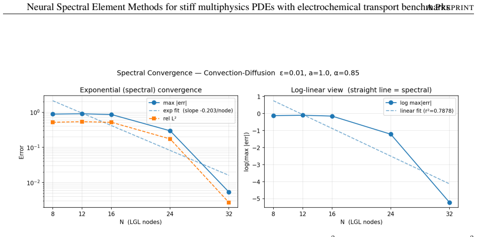
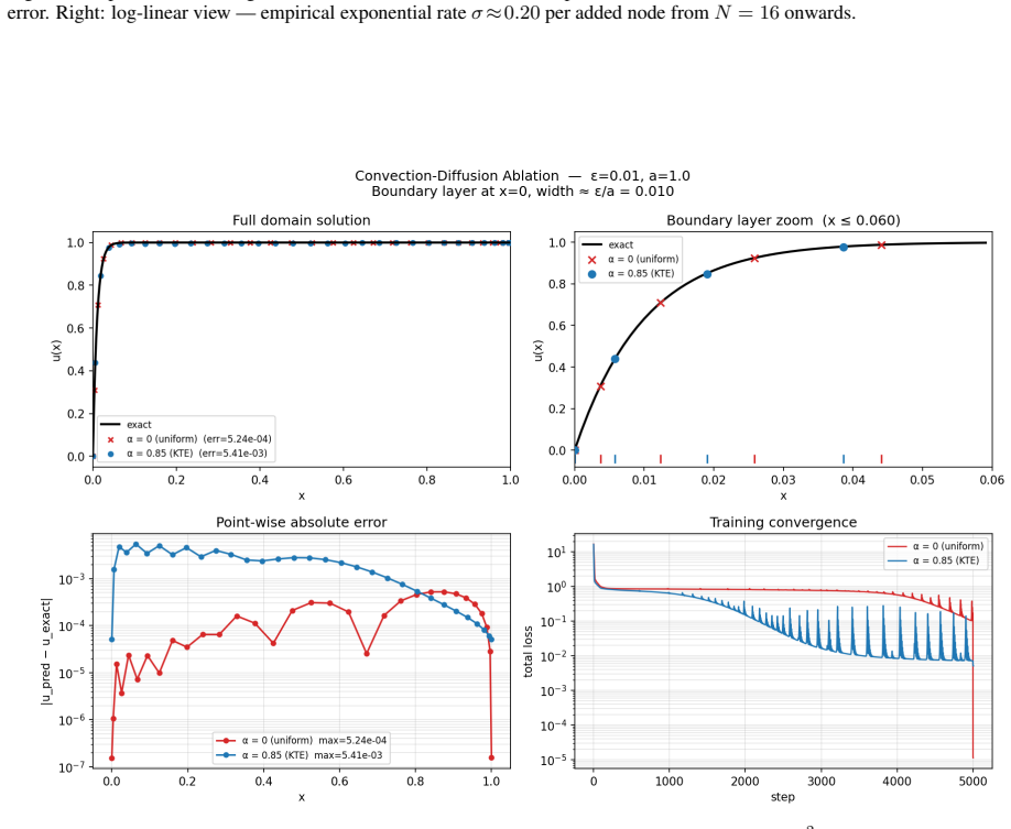
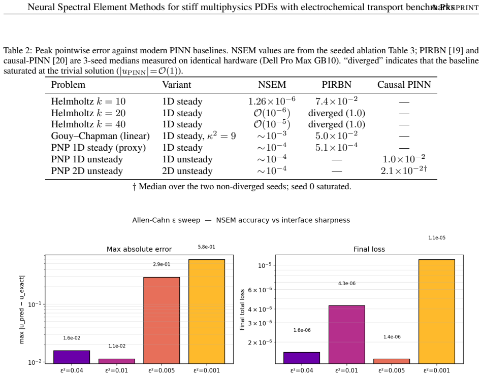
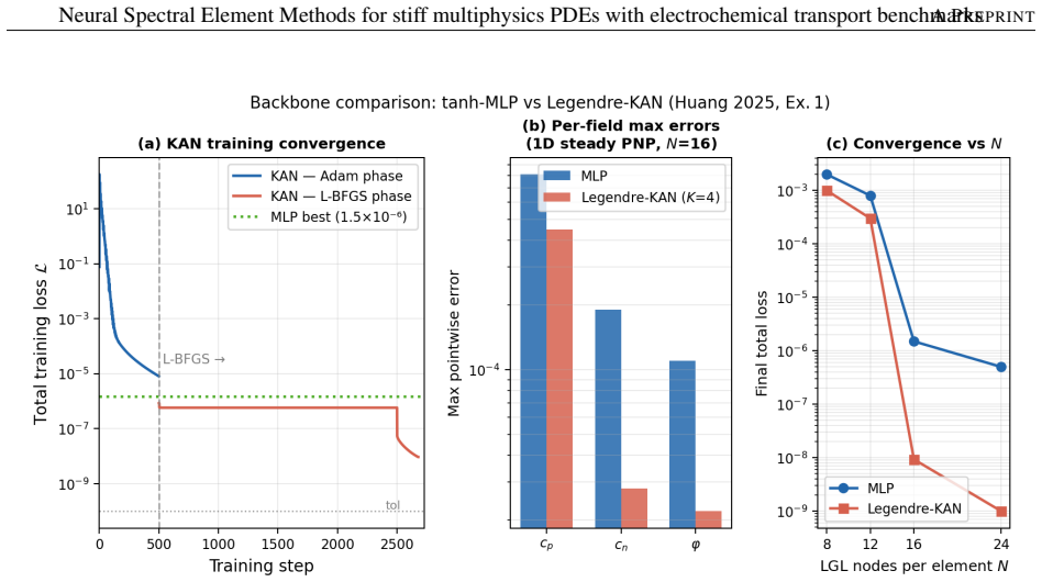
The Neural Spectral Element Method evaluates each network only at fixed Legendre-Gauss-Lobatto quadrature nodes and replaces all derivative calls with precomputed spectral differentiation matrices. The resulting deterministic loss enables limited-memory BFGS to reach residuals of 10^-9 to 10^-10. A Kosloff-Tal-Ezer coordinate map resolves electrochemical boundary layers, while a mesh-free neural mortar framework couples multi-element domains. On the four-example Poisson-Nernst-Planck benchmark, NSEM attains 10^-4 to 10^-7 relative pointwise error with two orders of magnitude fewer collocation points than the adaptive-resampling PINN baseline.
What carries the argument
Precomputed spectral differentiation matrices at Legendre-Gauss-Lobatto nodes combined with the Kosloff-Tal-Ezer coordinate map inside a neural mortar framework.
If this is right
- Both tanh multilayer perceptrons and basis-aligned Legendre Kolmogorov-Arnold Networks achieve spectral accuracy within the same infrastructure.
- The KAN backbone requires roughly half the Adam steps to enter the L-BFGS basin on the 1D PNP benchmark.
- The method handles multi-element domains without a mesh through the neural mortar framework.
- Accuracy reaches 10^-4 to 10^-7 relative pointwise error on the PNP benchmarks.
Where Pith is reading between the lines
- Similar spectral-element ideas could reduce training costs for other stiff PDE problems in materials science.
- The deterministic loss might allow integration with traditional solvers for hybrid approaches.
- Extending the mortar framework could enable simulations of larger electrochemical systems like batteries.
Load-bearing premise
The precomputed spectral differentiation matrices and Kosloff-Tal-Ezer map resolve the electrochemical boundary layers accurately enough that the loss function has no quadrature or mapping errors preventing L-BFGS from reaching 10^-9 residuals.
What would settle it
Compare NSEM pointwise errors and required collocation points against a high-resolution traditional spectral element solver or an adaptive finite element method on the same four PNP examples.
Figures
read the original abstract
The Neural Spectral Element Method (NSEM) evaluates each network only at fixed Legendre-Gauss-Lobatto quadrature nodes and replaces all derivative calls with precomputed spectral differentiation matrices. The resulting deterministic loss enables limited-memory BFGS (L-BFGS) to reach residuals of 10^-9 to 10^-10. A Kosloff-Tal-Ezer coordinate map resolves electrochemical boundary layers, while a mesh-free neural mortar framework couples multi-element domains. On the four-example Poisson-Nernst-Planck (PNP) benchmark of Huang and co-workers, NSEM attains 10^-4 to 10^-7 relative pointwise error with two orders of magnitude fewer collocation points than the adaptive-resampling PINN baseline. Both a tanh multilayer perceptron (MLP) and a basis-aligned Legendre Kolmogorov-Arnold Network (KAN) backbone attain spectral accuracy within the same NSEM infrastructure, with the KAN requiring roughly half the Adam steps to enter the L-BFGS basin of attraction on the 1D PNP benchmark.
Editorial analysis
A structured set of objections, weighed in public.
Referee Report
Summary. The manuscript introduces the Neural Spectral Element Method (NSEM) for stiff multiphysics PDEs, with focus on Poisson-Nernst-Planck (PNP) electrochemical transport. NSEM evaluates networks only at fixed Legendre-Gauss-Lobatto (LGL) nodes, replaces derivatives with precomputed spectral differentiation matrices, applies a Kosloff-Tal-Ezer coordinate map to cluster points near boundary layers, and employs a mesh-free neural mortar framework for multi-element coupling. On four PNP benchmark problems from Huang et al., it reports 10^{-4} to 10^{-7} relative pointwise errors using two orders of magnitude fewer collocation points than an adaptive-resampling PINN baseline, with L-BFGS driving the deterministic loss to 10^{-9}–10^{-10} residuals. Both tanh-MLP and basis-aligned Legendre KAN backbones are shown to reach spectral accuracy within the same framework.
Significance. If the central numerical claims hold after verification of the mapped operators, NSEM would constitute a meaningful advance by delivering deterministic, high-accuracy neural solvers that combine spectral-element efficiency with neural flexibility for problems featuring sharp electrochemical layers. The explicit use of precomputed differentiation matrices enabling reliable L-BFGS convergence, together with the direct benchmark comparison showing substantial reduction in degrees of freedom, are concrete strengths that could influence subsequent work on multiphysics PINN variants.
major comments (2)
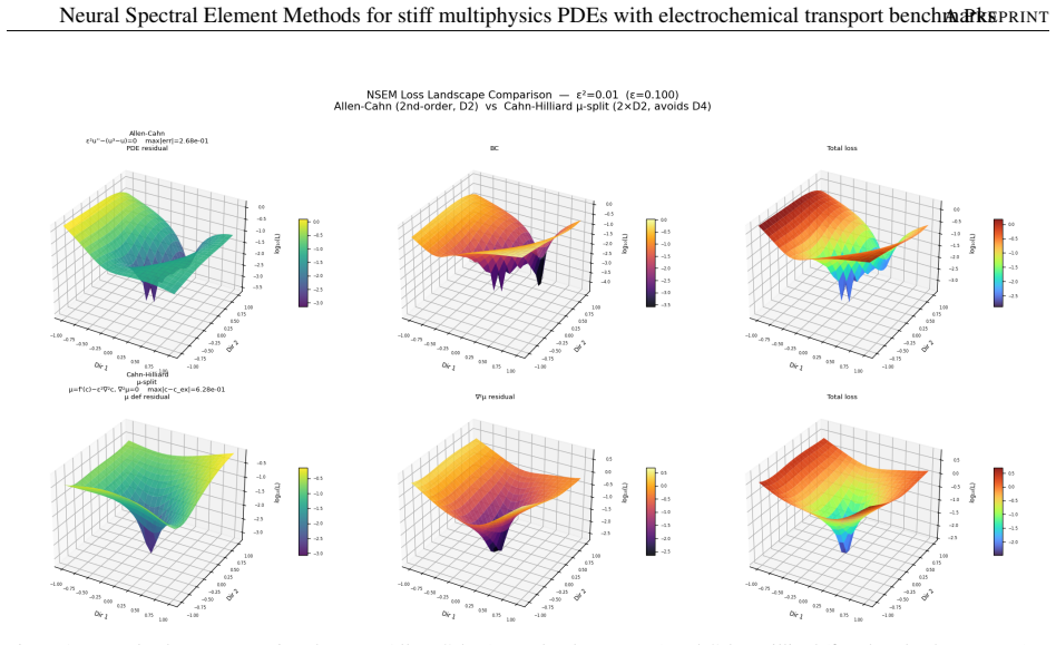
- [§2 (NSEM construction, coordinate-map paragraph)] §2 (NSEM construction, coordinate-map paragraph): the nonlinear Kosloff-Tal-Ezer map transforms the differential operators through the chain rule, producing variable-coefficient terms whose exact representation at the original fixed LGL nodes is not guaranteed by the unmapped precomputed differentiation matrices. The manuscript must demonstrate (via explicit error analysis or numerical verification) that any resulting quadrature or aliasing error lies below the claimed 10^{-9}–10^{-10} residual level; otherwise the deterministic-loss advantage and the reported pointwise accuracy cannot be taken as established.
- [Results section (PNP benchmark tables/figures)] Results section (PNP benchmark tables/figures): the two-order-of-magnitude reduction in collocation points relative to the adaptive PINN baseline is load-bearing for the efficiency claim, yet the manuscript does not report the precise number of points used by each method on each of the four examples or confirm that the pointwise error is evaluated on an identical, sufficiently dense reference grid independent of the training nodes.
minor comments (2)
- [§2.4] Notation for the neural mortar coupling should be introduced with an explicit equation showing how interface conditions are enforced in the loss; the current description is terse.
- [Figure captions] Figure captions for the error plots should state the exact norm and evaluation grid used for the reported relative pointwise errors.
Simulated Author's Rebuttal
We thank the referee for the thorough review and valuable feedback on our manuscript. We address the major comments point by point below, and we will incorporate revisions as indicated to improve the clarity and rigor of the presentation.
read point-by-point responses
-
Referee: [§2 (NSEM construction, coordinate-map paragraph)] §2 (NSEM construction, coordinate-map paragraph): the nonlinear Kosloff-Tal-Ezer map transforms the differential operators through the chain rule, producing variable-coefficient terms whose exact representation at the original fixed LGL nodes is not guaranteed by the unmapped precomputed differentiation matrices. The manuscript must demonstrate (via explicit error analysis or numerical verification) that any resulting quadrature or aliasing error lies below the claimed 10^{-9}–10^{-10} residual level; otherwise the deterministic-loss advantage and the reported pointwise accuracy cannot be taken as established.
Authors: We agree that an explicit demonstration is warranted for the mapped operators. In the revised manuscript we will add to §2 a short numerical verification subsection. This will compare the action of the chain-rule transformed differentiation matrices (evaluated at the fixed LGL nodes) against a reference spectral computation on a much finer grid for the specific Kosloff-Tal-Ezer stretching parameters used in the PNP benchmarks, confirming that the resulting operator error remains below 10^{-12} and therefore does not compromise the reported residual levels. revision: yes
-
Referee: [Results section (PNP benchmark tables/figures)] Results section (PNP benchmark tables/figures): the two-order-of-magnitude reduction in collocation points relative to the adaptive PINN baseline is load-bearing for the efficiency claim, yet the manuscript does not report the precise number of points used by each method on each of the four examples or confirm that the pointwise error is evaluated on an identical, sufficiently dense reference grid independent of the training nodes.
Authors: We concur that precise reporting is required to substantiate the efficiency claim. The revised manuscript will add a table in the Results section that lists, for each of the four PNP benchmarks, the exact number of collocation points employed by NSEM and by the adaptive-resampling PINN baseline. We will also state explicitly that all pointwise errors are computed on a fixed, independent reference grid of 100 000 uniformly spaced points that is denser than any training discretization used, and we will include pseudocode for the error-evaluation procedure. revision: yes
Circularity Check
No significant circularity; claims rest on direct construction rather than self-referential fits or citations
full rationale
The paper describes NSEM via precomputed LGL differentiation matrices, a Kosloff-Tal-Ezer map, and neural mortar coupling as an explicit algorithmic construction. Performance figures (10^-9–10^-10 residuals, 10^-4–10^-7 pointwise error) are presented as empirical outcomes on external PNP benchmarks, not as quantities algebraically forced by the method's own parameters or loss terms. No self-citation chains, uniqueness theorems, or ansatzes are invoked to justify core choices. The derivation therefore remains self-contained against external benchmarks, consistent with the default non-circular outcome.
Axiom & Free-Parameter Ledger
Reference graph
Works this paper leans on
-
[1]
Raissi M, Perdikaris P and Karniadakis G E 2019Journal of Computational Physics378686–707
-
[2]
Karniadakis G E, Kevrekidis I G, Lu L, Perdikaris P, Wang S and Yang L 2021Nature Reviews Physics3422–440
-
[3]
Krishnapriyan A S, Gholami A, Zhe S, Kirby R and Mahoney M W 2021 Characterizing possible failure modes in physics-informed neural networksAdvances in Neural Information Processing Systems (NeurIPS)vol 34 pp 26548–26560 (Preprint2109.01050)
arXiv 2021
-
[4]
Tancik M, Srinivasan P P, Mildenhall B, Fridovich-Keil S, Raghavan N, Singhal U, Ramamoorthi R, Barron J T and Ng R 2020 Fourier features let networks learn high-frequency functions in low-dimensional domains Advances in Neural Information Processing Systems (NeurIPS)vol 33 pp 7537–7547
2020
-
[5]
Rahaman N, Baratin A, Arpit D, Draxler F, Lin M, Hamprecht F A, Bengio Y and Courville A 2019 On the spectral bias of neural networksInternational Conference on Machine Learning (ICML)(Preprint 1806.08734)
Pith/arXiv arXiv 2019
-
[6]
Mishra S and Molinaro R 2023IMA Journal of Numerical Analysis431–43 (Preprint2006.16144)
-
[7]
Mishra S and Molinaro R 2022IMA Journal of Numerical Analysis42981–1022 (Preprint2007.01138) 23 Neural Spectral Element Methods for stiff multiphysics PDEs with electrochemical transport benchmarksA PREPRINT
-
[8]
Liu Z, Wang Y , Vaidya S, Ruehle F, Halverson J, Soljaˇci´c M, Hou T Y and Tegmark M 2024Transactions on Machine Learning ResearchISSN 2835-8856 (Preprint2404.19756)
-
[9]
Patera A T 1984Journal of Computational Physics54468–488
-
[10]
Karniadakis G E and Sherwin S J 2005Spectral/hp Element Methods for Computational Fluid Dynamics2nd ed (Oxford University Press)
-
[11]
Komatitsch D and Tromp J 1999Geophysical Journal International139806–822
-
[12]
Jagtap A D and Karniadakis G E 2020Communications in Computational Physics282002–2041 (Preprint 2004.02518)
arXiv 2041
-
[13]
Moseley B, Markham A and Nissen-Meyer T 2023Advances in Computational Mathematics49(Preprint 2107.07871)
-
[14]
Kharazmi E, Zhang Z and Karniadakis G E 2021Computer Methods in Applied Mechanics and Engineering374 113547 (Preprint2003.05385)
-
[15]
Anandh T, Ghose D, Jain H and Ganesan S 2024SIAM Journal on Scientific Computing46A3881–A3908 (Preprint2404.12063)
-
[16]
Du Y , Chalapathi N and Krishnapriyan A 2024 Neural spectral methods: Self-supervised learning in the spectral domainInternational Conference on Learning Representations (ICLR)(Preprint2312.05225)
arXiv 2024
-
[17]
Yu T, Qi Y , Oseledets I and Chen S 2025Journal of Computational and Applied Mathematics(Preprint 2408. 16414)
-
[18]
Shukla K, Zou Z, Chan C H, Pandey A, Wang Z and Karniadakis G E 2024Computer Methods in Applied Mechanics and Engineering433117498 (Preprint2407.21217)
-
[19]
Anagnostopoulos S J, Toscano J D, Stergiopulos N and Karniadakis G E 2024Computer Methods in Applied Mechanics and Engineering421116805 (Preprint2307.00379)
-
[20]
Wang S, Sankaran S and Perdikaris P 2024Computer Methods in Applied Mechanics and Engineering421116813 (Preprint2203.07404)
-
[21]
Wang Y , Sun J, Bai J, Anitescu C, Eshaghi M S, Zhuang X, Rabczuk T and Liu Y 2024Computer Methods in Applied Mechanics and Engineering(Preprint2406.11045)
-
[22]
Zhang Z, Xiong X, Zhang S, Wang W, Zhong Y , Yang C and Yang X 2025Expert Systems with Applications (Preprint2406.08992)
-
[23]
SS S and R G 2024 Chebyshev polynomial-based Kolmogorov–Arnold networks: An efficient architecture for nonlinear function approximation arXiv preprint arXiv:2405.07200 (Preprint2405.07200)
arXiv 2024
-
[24]
Guo C, Sun L, Li S, Yuan Z and Wang C 2024 Physics-informed Kolmogorov–Arnold network with Chebyshev polynomials for fluid mechanics arXiv preprint arXiv:2411.04516 (Preprint2411.04516)
arXiv 2024
-
[25]
Berrut J P and Trefethen L N 2004SIAM Review46501–517
-
[26]
Trefethen L N 2000Spectral Methods in MATLAB(Philadelphia: SIAM)
-
[27]
Boyd J P 2001Chebyshev and Fourier Spectral Methods2nd ed (New York: Dover)
-
[28]
Light J C, Hamilton I P and Lill J V 1985Journal of Chemical Physics821400
-
[29]
Colbert D T and Miller W H 1992Journal of Chemical Physics961982–1991
1991
-
[30]
Wang Z, Hao S, Zhang Y and Zhang L 2024SIAM Journal on Numerical Analysis621702–1720 (Preprint 2405.14099)
-
[31]
Kosloff D and Tal-Ezer H 1993Journal of Computational Physics104457–469
-
[32]
XIed Brezis H and Lions J L (Pitman Research Notes in Mathematics) pp 13–51
Bernardi C, Maday Y and Patera A T 1994 A new nonconforming approach to domain decomposition: The mortar element methodNonlinear Partial Differential Equations and Their Applications, Collège de France Seminar, vol. XIed Brezis H and Lions J L (Pitman Research Notes in Mathematics) pp 13–51
1994
-
[33]
Lacour C and Maday Y 1997BIT Numerical Mathematics37720–738
-
[34]
Chen W, Howard A A and Stinis P 2025Journal of Computational Physics(Preprint 2407.01613) URL https://www.sciencedirect.com/science/article/pii/S0021999125005091
-
[35]
Liu D C and Nocedal J 1989Mathematical Programming45503–528
-
[36]
Byrd R H, Lu P, Nocedal J and Zhu C 1995SIAM Journal on Scientific Computing161190–1208 24 Neural Spectral Element Methods for stiff multiphysics PDEs with electrochemical transport benchmarksA PREPRINT
-
[37]
Doumèche N, Biau G and Boyer C 2023 On the convergence of PINNs arXiv preprint arXiv:2305.01240 (Preprint 2305.01240)
arXiv 2023
-
[38]
Newman J and Thomas-Alyea K E 2004Electrochemical Systems3rd ed (Wiley)
-
[39]
Bard A J and Faulkner L R 2001Electrochemical Methods: Fundamentals and Applications2nd ed (Wiley)
-
[40]
Bazant M Z, Thornton K and Ajdari A 2004Physical Review E70021506 (Preprintcond-mat/0401118)
-
[41]
Huang X, Wang F, Zhang B and Liu H 2025Mathematics and Computers in Simulation237231–246 (Preprint 2402.01768)
-
[42]
Wang S, Yu X and Perdikaris P 2022Journal of Computational Physics449110768 (Preprint2007.14527)
-
[43]
Macdonald J R 1953Physical Review924–17
-
[44]
Lasia A 2014Electrochemical Impedance Spectroscopy and Its Applications2nd ed (Springer)
-
[45]
Orazem M E and Tribollet B 2017Electrochemical Impedance Spectroscopy2nd ed (Wiley (ECS Series))
-
[46]
Doyle M, Fuller T F and Newman J 1993Journal of The Electrochemical Society1401526–1533 25
discussion (0)
Sign in with ORCID, Apple, or X to comment. Anyone can read and Pith papers without signing in.