Neural Parameter Calibration for Finite-State Mean Field Games
Pith reviewed 2026-06-26 06:21 UTC · model grok-4.3
The pith
A neural network framework learns parameters of finite-state mean field games directly from observed population dynamics using implicit differentiation.
A machine-rendered reading of the paper's core claim, the machinery that carries it, and where it could break.
Core claim
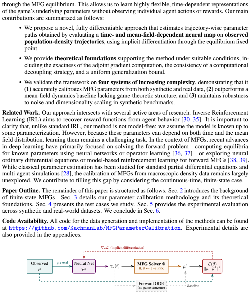
The authors present a neural network-based framework for learning parametric, finite-state MFGs from observed population dynamics. They formulate the parameter calibration as an inverse problem and use implicit differentiation to backpropagate through the games' equilibrium. The approach is fully differentiable and supports estimation of flexible trajectory-wise parameter paths, including state- and time-dependent specifications, without requiring observations of individual agents' actions or rewards. They prove the exactness of the gradient computation in a discrete-time formulation.
What carries the argument
Implicit differentiation through the mean-field equilibrium to enable backpropagation for parameter learning in finite-state games.
If this is right
- Enables estimation of state- and time-dependent parameter paths from population data alone.
- Supports fully differentiable calibration without access to individual agent actions or rewards.
- Provides exact gradient computation in discrete-time formulations of the inverse problem.
- Applies to systems ranging from synthetic linear-quadratic benchmarks to real-world urban mobility datasets.
Where Pith is reading between the lines
- If the framework recovers parameters accurately on real mobility data, it could support dynamic recalibration in transportation planning models.
- The method's differentiability may allow integration into larger learning pipelines for multi-agent systems.
Load-bearing premise
The observed population dynamics are generated exactly by the mean-field equilibrium of a finite-state game, and the parameters of that game are recoverable through the inverse problem formulation.
What would settle it
Running the method on synthetic data generated from a known finite-state mean field game and checking whether the recovered parameters match the ground-truth values within numerical error.
Figures
read the original abstract
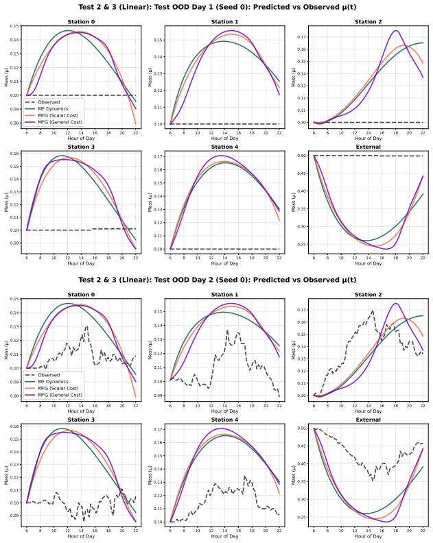
Mean field games efficiently approximate a very large population of strategic agents. While these games can aid the understanding of complex systems, their deployment in real-world settings is challenged by the specification of their parameters: mean field games (MFGs) often involve hidden preferences, constraints, and interactions that can rarely be theoretically derived or directly observed. To address this gap, we present a neural network-based framework for learning parametric, finite-state MFGs from observed population dynamics. To do so, we formulate the parameter calibration as an inverse problem and use implicit differentiation to backpropagate through the games' equilibrium. The resulting approach is fully differentiable and enables us to estimate flexible trajectory-wise parameter paths, including state- and time-dependent specifications without requiring observations of the individual agents' actions or rewards. We provide a proof for the exactness of the gradient computation in a discrete-time formulation. We validate our framework through numerical experiments across four systems of increasing complexity, ranging from synthetic linear-quadratic benchmarks to real-world urban mobility datasets.
Editorial analysis
A structured set of objections, weighed in public.
Referee Report
Summary. The paper introduces a neural network framework to calibrate parameters of finite-state mean field games from observed population dynamics by casting the task as an inverse problem and applying implicit differentiation through an equilibrium solver. It claims a proof that the resulting gradients are exact in the discrete-time case, supports estimation of flexible state- and time-dependent parameter trajectories, and validates the approach on four systems ranging from linear-quadratic benchmarks to real urban mobility data, without requiring individual agent actions or rewards.
Significance. If the gradient exactness result holds under the stated conditions and the method recovers parameters reliably from aggregate data, the framework would enable data-driven deployment of MFGs in settings where parameters cannot be derived theoretically, which is a meaningful contribution to applied game-theoretic modeling.
major comments (2)
- [discrete-time formulation / implicit differentiation proof] The proof of gradient exactness (referenced in the abstract and developed in the discrete-time formulation section): the argument invokes the implicit function theorem on the fixed-point map F(μ, θ) = 0 but does not state or verify the required invertibility of ∂F/∂μ at the solution. This condition is load-bearing for the central claim of exact backpropagation, as non-invertibility can arise in finite-state MFGs with non-strictly monotone costs or multiple equilibria.
- [Section 5] Validation experiments (Section 5, real-world urban mobility dataset): the reported fits assume the observed dynamics are generated exactly by a unique mean-field equilibrium whose parameters are recoverable; no diagnostic is provided for Jacobian conditioning or equilibrium uniqueness, which directly affects whether the claimed exact gradients are realized on the real data.
minor comments (2)
- [Method overview] Notation for the equilibrium map and the neural parameterization of θ(t,s) should be introduced with explicit dimensions and domains to avoid ambiguity when describing the trajectory-wise estimation.
- [Numerical experiments] The four validation systems are described at a high level; adding a table summarizing the state space size, time horizon, and parameter dimensionality for each would improve reproducibility.
Simulated Author's Rebuttal
We thank the referee for the careful reading and constructive feedback on our manuscript. We address each major comment below, providing clarifications and indicating where revisions will be made to strengthen the presentation.
read point-by-point responses
-
Referee: The proof of gradient exactness (referenced in the abstract and developed in the discrete-time formulation section): the argument invokes the implicit function theorem on the fixed-point map F(μ, θ) = 0 but does not state or verify the required invertibility of ∂F/∂μ at the solution. This condition is load-bearing for the central claim of exact backpropagation, as non-invertibility can arise in finite-state MFGs with non-strictly monotone costs or multiple equilibria.
Authors: We agree that the invertibility condition is essential for the implicit function theorem application. The discrete-time analysis in the manuscript is developed under the standard MFG assumptions of strict monotonicity in the running and terminal costs, which guarantee local invertibility of ∂F/∂μ at an isolated equilibrium (see e.g. the contraction mapping arguments in the existence proofs). However, the current text does not explicitly restate this condition before invoking the theorem. We will revise the discrete-time section to include a clear statement of the required Jacobian invertibility, note that the result holds locally around the observed equilibrium, and add a remark on the implications of multiple equilibria. This will be revision_made = 'yes'. revision: yes
-
Referee: Validation experiments (Section 5, real-world urban mobility dataset): the reported fits assume the observed dynamics are generated exactly by a unique mean-field equilibrium whose parameters are recoverable; no diagnostic is provided for Jacobian conditioning or equilibrium uniqueness, which directly affects whether the claimed exact gradients are realized on the real data.
Authors: We acknowledge the point: real-world data precludes direct verification of uniqueness or conditioning. In the urban mobility experiments we mitigate this by (i) initializing the parameter network from multiple random seeds and observing convergence to statistically indistinguishable trajectories, and (ii) reporting low validation loss on held-out time steps. These provide indirect support but are not formal diagnostics. We will add a short limitations paragraph in Section 5 discussing the assumption of a unique equilibrium and suggesting practical checks (e.g., monitoring the norm of the implicit Jacobian during training). This constitutes a partial revision. revision: partial
Circularity Check
No significant circularity detected
full rationale
The paper formulates parameter calibration as an inverse problem solved via neural networks and implicit differentiation through the MFG equilibrium map, with an explicit proof supplied for gradient exactness in the discrete-time case. This structure does not reduce any claimed prediction or parameter estimate to a quantity defined by the fit itself, nor does it rely on self-citations, imported uniqueness theorems, or ansatzes that are load-bearing for the central result. The derivation remains self-contained against external benchmarks such as the implicit function theorem applied to the fixed-point equation, with no evidence of self-definitional steps or fitted inputs renamed as predictions.
Axiom & Free-Parameter Ledger
axioms (1)
- domain assumption Observed population dynamics are generated by the mean-field equilibrium of the finite-state game
Reference graph
Works this paper leans on
-
[1]
Mean Field Games.Japanese Journal of Mathemat- ics, 2:229–260, 03 2007
Jean-Michel Lasry and Pierre-Louis Lions. Mean Field Games.Japanese Journal of Mathemat- ics, 2:229–260, 03 2007. doi:10.1007/s11537-007-0657-8
-
[2]
Minyi Huang, Roland P. Malhamé, and Peter E. Caines. Large population stochastic dynamic games: closed-loop McKean-Vlasov systems and the Nash certainty equivalence principle.Com- munications in Information & Systems, 6(3):221 – 252, 2006. doi:10.4310/CIS.2006.v6.n3.a5
-
[3]
Geoffroy Chevalier, Jerome Le Ny, and Roland Malhamé.A micro-macro traffic model based on Mean-Field Games, pages 1983–1988. IEEE, 2015. doi:10.1109/ACC.2015.7171024. 10
-
[4]
A Mean Field Games approach for multi-lane traffic management
Adriano Festa and Simone Göttlich. A mean field game approach for multi-lane traffic manage- ment.IFAC-PapersOnLine, 51(32):793–798, 2018. doi:10.48550/arXiv.1711.04116
work page internal anchor Pith review Pith/arXiv arXiv doi:10.48550/arxiv.1711.04116 2018
-
[5]
Stabilizing Traffic via Autonomous Vehicles: A Continuum Mean Field Game Approach
Kuang Huang, Xuan Di, Qiang Du, and Xi Chen. Stabilizing Traffic via Autonomous Vehicles: A Continuum Mean Field Game Approach. In2019 IEEE Intelligent Transportation Systems Conference (ITSC), pages 3269–3274, 2019. doi:10.1109/ITSC.2019.8917021
-
[6]
Takashi Tanaka, Ehsan Nekouei, Ali Reza Pedram, and Karl Henrik Johansson. Linearly Solvable Mean-Field Traffic Routing Games.IEEE Transactions on Automatic Control, 66(2): 880–887, 2021. doi:10.1109/TAC.2020.2986195
-
[7]
Emma Hubert and Gabriel Turinici. Nash-MFG equilibrium in a SIR model with time dependent newborn vaccination.Ricerche di matematica, 67(1):227–246, 2018. doi:10.1007/s11587-018- 0365-0
-
[8]
A Mean Field Game Analysis of SIR Dynamics with Vaccination.Probability in the Engineering and Informational Sciences, 36(2):482–499,
Josu Doncel, Nicolas Gast, and Bruno Gaujal. A Mean Field Game Analysis of SIR Dynamics with Vaccination.Probability in the Engineering and Informational Sciences, 36(2):482–499,
-
[9]
doi:10.1017/S0269964820000522
-
[10]
Wonjun Lee, Siting Liu, Hamidou Tembine, Wuchen Li, and Stanley Osher. Controlling Propagation of Epidemics via Mean-Field Control.SIAM Journal on Applied Mathematics, 81 (1):190–207, 2021. doi:10.1137/20M1342690
-
[11]
Carmona, Gökçe Dayanıklı, and Mathieu Laurière
Alexander Aurell, René. Carmona, Gökçe Dayanıklı, and Mathieu Laurière. Finite state graphon games with applications to epidemics.Dyn Games Appl, 12(1):49–81, 2022. ISSN 2153-0785 (Print) 2153-0785. doi:10.1007/s13235-021-00410-2
-
[12]
Behavioral patterns and mean-field games in epidemiological models.arXiv preprint, 2025
Finnegan Buckley and Alexander Vladimirsky. Behavioral patterns and mean-field games in epidemiological models.arXiv preprint, 2025. doi:10.48550/arXiv.2512.20547
-
[13]
Huaning Liu, Junke Yang, Soren L. Larsen, Pamela P. Martinez, and Gökçe Dayanıklı. Incorpo- rating Authority Perception, Economic Status, and Behavioral Response in Infectious Disease Control.arXiv preprint, 2025. doi:10.48550/arXiv.2512.23188
-
[14]
Modeling Epidemic Spread with Strategic Vaccination and Socialization: a Mean Field Game Analysis
Huaning Liu and Gökçe Dayanıklı. Modeling Epidemic Spread with Strategic Vac- cination and Socialization: a Mean Field Game Analysis.arXiv preprint, 2026. doi:10.48550/arXiv.2604.22946
work page internal anchor Pith review Pith/arXiv arXiv doi:10.48550/arxiv.2604.22946 2026
-
[15]
Mean field game of controls and an application to trade crowding.Mathematics and Financial Economics, 12(3):335–363, 2018
Pierre Cardaliaguet and Charles-Albert Lehalle. Mean field game of controls and an application to trade crowding.Mathematics and Financial Economics, 12(3):335–363, 2018. ISSN 1862-
2018
-
[16]
doi:10.1007/s11579-017-0206-z
-
[17]
Applications of Mean Field Games in Financial Engineering and Economic Theory.arXiv preprint, 2020
Rene Carmona. Applications of Mean Field Games in Financial Engineering and Economic Theory.arXiv preprint, 2020. doi:10.48550/arXiv.2012.05237
-
[18]
Cambridge University Press, 2023
René Carmona and Mathieu Laurière.Deep Learning for Mean Field Games and Mean Field Control with Applications to Finance, page 369–392. Cambridge University Press, 2023. doi:10.1017/9781009028943.021
-
[19]
Kolokoltsov and Alain Bensoussan
Vassili N. Kolokoltsov and Alain Bensoussan. Mean-Field-Game Model for Botnet Defense in Cyber-Security.Applied Mathematics & Optimization, 74(3):669–692, 2016. ISSN 1432-0606. doi:10.1007/s00245-016-9389-6
-
[20]
Chengshan Qian, Xue Li, Ning Sun, and Yuqing Tian. Data Security Defense and Algorithm for Edge Computing Based on Mean Field Game.Journal of Cybersecurity, 2(2):97, 2020. doi:10.32604/jcs.2020.010548
-
[21]
Shigen Shen, Chenpeng Cai, Yizhou Shen, Xiaoping Wu, Wenlong Ke, and Shui Yu. Joint mean-field game and multiagent asynchronous advantage actor-critic for edge intelligence-based iot malware propagation defense.IEEE Transactions on Dependable and Secure Computing, 22(4):3824–3838, 2025. doi:10.1109/TDSC.2025.3542104
-
[22]
Springer Briefs in Mathematics, 2013
Alain Bensoussan, Jens Frehse, and Phillip Yam.Mean Field Games and Mean Field Type Control Theory. Springer Briefs in Mathematics, 2013. doi:10.1007/978-1-4614-8508-7
-
[23]
Probability Theory and Stochastic Modelling
René Carmona and François Delarue.Probabilistic theory of mean field games with applications I. Probability Theory and Stochastic Modelling. Springer Cham, 2018. ISBN 978-3-319-58920-
2018
-
[24]
doi:10.1007/978-3-319-58920-6
-
[25]
Safe Control Synthesis via Input Constrained Control Barrier Func- tions,
Berkay Anahtarci, Can Deha Kariksiz, and Naci Saldi. Learning in Discrete-time Average-cost Mean-field Games. In2021 60th IEEE Conference on Decision and Control (CDC), pages 3048–3053. IEEE, 2021. doi:10.1109/CDC45484.2021.9682954
-
[26]
Bora Yongacoglu, Gürdal Arslan, and Serdar Yüksel. Independent learning and subjectivity in mean-field games. In2022 IEEE 61st Conference on Decision and Control (CDC), pages 2845–2850. IEEE, 2022. doi:10.1109/CDC51059.2022.9992399. 11
-
[27]
Policy Mirror Ascent for Efficient and Independent Learning in Mean Field Games
Batuhan Yardim, Semih Cayci, Matthieu Geist, and Niao He. Policy Mirror Ascent for Efficient and Independent Learning in Mean Field Games. InInternational Conference on Machine Learning, pages 39722–39754. PMLR, 2023. doi:10.48550/arXiv.2212.14449
-
[28]
Gomes, Joana Mohr, and Rafael Rigao Souza
Diogo A. Gomes, Joana Mohr, and Rafael Rigao Souza. Continuous Time Finite State Mean Field Games.Applied Mathematics & Optimization, 68(1):99–143, 2013. doi:10.1007/s00245- 013-9202-8
-
[29]
Adaptive Consensus and Parameter Estimation of Multiagent Systems With an Uncertain Leader.IEEE Transactions on Automatic Control, 66(9):4393–4400,
Shimin Wang and Xiangyu Meng. Adaptive Consensus and Parameter Estimation of Multiagent Systems With an Uncertain Leader.IEEE Transactions on Automatic Control, 66(9):4393–4400,
-
[30]
doi:10.1109/TAC.2020.3046215
-
[31]
Efficient Parameter Tuning for Multi-agent Simulation Using Deep Reinforcement Learning
Masanori Hirano and Kiyoshi Izumi. Efficient Parameter Tuning for Multi-agent Simulation Using Deep Reinforcement Learning. In2022 13th International Congress on Advanced Applied Informatics Winter (IIAI-AAI-Winter), pages 130–137, 2022. doi:10.1109/IIAI-AAI- Winter58034.2022.00035
-
[32]
Thomas Gaskin, Grigorios A. Pavliotis, and Mark Girolami. Neural parameter calibration for large-scale multiagent models.Proceedings of the National Academy of Sciences, 120(7): e2216415120, 2023. doi:10.1073/pnas.2216415120
-
[33]
Stefano Giampiccolo, Federico Reali, Anna Fochesato, Giovanni Iacca, and Luca Marchetti. Robust parameter estimation and identifiability analysis with hybrid neural ordinary differential equations in computational biology.npj Systems Biology and Applications, 10(1):139, 2024. ISSN 2056-7189. doi:10.1038/s41540-024-00460-3
-
[34]
Individual-Level Inverse Re- inforcement Learning for Mean Field Games
Yang Chen, Libo Zhang, Jiamou Liu, and Shuyue Hu. Individual-Level Inverse Re- inforcement Learning for Mean Field Games. InProceedings of the 21st Interna- tional Conference on Autonomous Agents and Multiagent Systems, pages 253–262, 2022. doi:10.48550/arXiv.2202.06401
-
[35]
Adversarial Inverse Reinforcement Learning for Mean Field Games.arXiv preprint, 2021
Yang Chen, Libo Zhang, Jiamou Liu, and Michael Witbrock. Adversarial Inverse Reinforcement Learning for Mean Field Games.arXiv preprint, 2021. doi:10.48550/arXiv.2104.14654
-
[37]
Berkay Anahtarci, Can Deha Kariksiz, and Naci Saldi. Maximum Causal Entropy IRL in Mean-Field Games and GNEP Framework for Forward RL.Journal of Machine Learning Research, 26(121):1–40, 2025. doi:10.48550/arXiv.2401.06566
-
[38]
Inverse Reinforcement Learning for Mean-field Games with Average Reward Criterion
¸ Sevket Kaan Alkır and Naci Saldi. Inverse Reinforcement Learning for Mean-field Games with Average Reward Criterion. In2025 IEEE 64th Conference on Decision and Control (CDC), pages 7272–7277. IEEE, 2025. doi:10.1109/CDC57313.2025.11312818
-
[39]
Berkay Anahtarci, Can Deha Kariksiz, and Naci Saldi. Kernel Based Maximum En- tropy Inverse Reinforcement Learning for Mean-Field Games.arXiv preprint, 2025. doi:10.48550/arXiv.2507.14529
-
[40]
Deep backward and Galerkin methods for the finite state master equation.J
Asaf Cohen, Mathieu Laurière, and Ethan Zell. Deep backward and Galerkin methods for the finite state master equation.J. Mach. Learn. Res., 25(1), January 2024. ISSN 1532-4435. doi:10.48550/arXiv.2403.04975
-
[41]
Operator Learning for Families of Finite-State Mean-Field Games.arXiv preprint, 2026
William Hofgard, Asaf Cohen, and Mathieu Laurière. Operator Learning for Families of Finite-State Mean-Field Games.arXiv preprint, 2026. doi:10.48550/arXiv.2602.13169
-
[42]
Anna C. M. Thöni, Yoram Bachrach, and Tal Kachman. Neural Mean-Field Games: Extending Mean-Field Game Theory with Neural Stochastic Differential Equations.arXiv preprint, 2026. doi:10.48550/arXiv.2504.13228
work page internal anchor Pith review Pith/arXiv arXiv doi:10.48550/arxiv.2504.13228 2026
-
[43]
Model-Based RL for Mean-Field Games is not Statistically Harder than Single-Agent RL
Jiawei Huang, Niao He, and Andreas Krause. Model-Based RL for Mean-Field Games is not Statistically Harder than Single-Agent RL. InForty-first International Conference on Machine Learning, 2024. doi:10.48550/arXiv.2402.05724
-
[44]
Kolokoltsov.Nonlinear Markov Processes and Kinetic Equations
Vassili N. Kolokoltsov.Nonlinear Markov Processes and Kinetic Equations. Cambridge Tracts in Mathematics. Cambridge University Press, 2010. doi:10.1017/CBO9780511760303
-
[45]
In: Proceed- ings of the 6th International Conference on Information Hiding
Peter E. Caines, Minyi Huang, and Roland P. Malhamé.Mean Field Games, pages 1–28. Springer International Publishing, Cham, 2017. ISBN 978-3-319-27335-8. doi:10.1007/978-3- 319-27335-8_7-1
-
[46]
Adam: A Method for Stochastic Optimization
Diederik P. Kingma and Jimmy Ba. Adam: A Method for Stochastic Optimization.CoRR, abs/1412.6980, 2014. doi:10.48550/arXiv.1412.6980
work page internal anchor Pith review Pith/arXiv arXiv doi:10.48550/arxiv.1412.6980 2014
-
[47]
Elisabetta Carlini and Francisco J. Silva. A Fully Discrete Semi-Lagrangian Scheme for a First Order Mean Field Game Problem.SIAM Journal on Numerical Analysis, 52(1):45–67, 2014. doi:10.1137/120902987. 12
-
[48]
Zico Kolter, and Vladlen Koltun
Shaojie Bai, J. Zico Kolter, and Vladlen Koltun. Deep Equilibrium Models. InAdvances in Neural Information Processing Systems, volume 32, 2019. doi:10.48550/arXiv.1909.01377
-
[49]
Efficient and Modular Implicit Dif- ferentiation
Mathieu Blondel, Quentin Berthet, Marco Cuturi, Roy Frostig, Stephan Hoyer, Felipe Llinares- López, Fabian Pedregosa, and Jean-Philippe Vert. Efficient and Modular Implicit Dif- ferentiation. InAdvances in Neural Information Processing Systems, volume 35, 2022. doi:10.48550/arXiv.2105.15183
-
[50]
Numerical Methods for Mean Field Games and Mean Field Type Control
Mathieu Laurière. Numerical Methods for Mean Field Games and Mean Field Type Control. In Proc. Sympos. Appl. Math., volume 78, page 221–282. Amer. Math. Soc., Providence, RI, 2021. doi:10.48550/arXiv.2106.06231
-
[51]
William Ogilvy Kermack and Anderson G. McKendrick. A contribution to the mathematical theory of epidemics.Proceedings of the royal society of london. Series A, Containing papers of a mathematical and physical character, 115(772):700–721, 1927. doi:10.1098/rspa.1927.0118
-
[52]
Alexander Aurell, René Carmona, Gökçe Dayanıklı, and Mathieu Laurière. Optimal Incentives to Mitigate Epidemics: A Stackelberg Mean Field Game Approach.SIAM Journal on Control and Optimization, 60(2):S294–S322, 2022. doi:10.1137/20M1377862
-
[53]
Centers for Disease Control and Prevention
U.S. Centers for Disease Control and Prevention. Percent positivity of Respiratory Viruses as reported on the National Respiratory and Enteric Virus Surveillance System (NREVSS) Dashboard. https://www.cdc.gov/nrevss/php/dashboard/index.html/, 2026. The data falls under the Public Domain (U.S. Government). Data retrieved on May 4, 2026
2026
-
[54]
Citi Bike Trip Histories
Citi Bike. Citi Bike Trip Histories. https://citibikenyc.com/system-data, 2026. Li- censed under the NYCBS Data Use Policy. Data retrieved on May 4, 2026
2026
-
[55]
Probabilistic approach to finite state mean field games
Alekos Cecchin and Markus Fischer. Probabilistic approach to finite state mean field games. Applied Mathematics & Optimization, 81:253–300, 2020. doi:10.1007/s00245-018-9488-7
-
[56]
Joseph Sung, Sheung Chi Phillip Yam, and Siu-Pang Yung
Alain Bensoussan, K.C. Joseph Sung, Sheung Chi Phillip Yam, and Siu-Pang Yung. Linear- Quadratic Mean Field Games.Journal of Optimization Theory and Applications, 169(2): 496–529, 2016. doi:10.1007/s10957-015-0819-4
-
[57]
JAX: composable transformations of Python+NumPy programs, 2018
James Bradbury, Roy Frostig, Peter Hawkins, Matthew James Johnson, Yash Katariya, Chris Leary, Dougal Maclaurin, George Necula, Adam Paszke, Jake VanderPlas, Skye Wanderman- Milne, and Qiao Zhang. JAX: composable transformations of Python+NumPy programs, 2018. URLhttp://github.com/jax-ml/jax. 13 A Picard Iteration for Solving MFGs Picard iteration is a fi...
2018
-
[58]
and R(θ) =E P[ℓ(θ;µ obs, µ0)]. Then, for any δ∈(0,1) and ϵ >0 , with probability at least 1−δ over the draw of S, for all θ∈Θ : R(θ)≤ ˆR(θ) + 2Lℓϵ+B r log(2N(ϵ,Θ)/δ) 2M ,(B.5) where N(ϵ,Θ) denotes the ϵ-covering number of Θ in the ℓ2 norm, CN,d := p dT(1 + 1/N), and Lℓ = 2 √ B·C N,d · LΞ,γ 1−κ ·L φ,θ is the Lipschitz constant ofℓwith respect toθ. 17 For f...
-
[59]
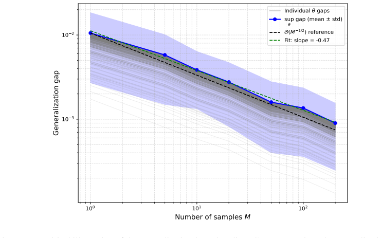
Gray curves show the generalization gap |R(θ)− ˆRM(θ)| averaged over S= 100 subsamples for each of the 500 randomly sampled parameters θ∈Θ
Worst-case loss bound B.The bound assumes ℓ(θ;µ obs)≤B for all θ∈Θ and all possible observations, where B= 2T(1 + 1/N) bounds the squared L2 distance between any two 19 100 101 102 Number of samples M 10 3 10 2 Generalization gap Individual gaps sup gap (mean ± std) (M 1/2) reference Fit: slope = -0.47 Figure 7: Empirical illustration of the generalizatio...
-
[60]
In practice, the loss function varies appreciably only over a much smaller effective region around the true parameterθ∗
Parameter space diameter D.The covering number N(ϵ,Θ)≤(1 + 2D/ϵ) p grows polynomially with the diameter D= diam(Θ) of the full parameter space. In practice, the loss function varies appreciably only over a much smaller effective region around the true parameterθ∗
-
[61]
Distribution-free nature.The Hoeffding–union bound argument holds foranydata-generating distribution over initial conditions µ0. It cannot exploit the specific concentration properties of the Dirichlet distribution or the smoothness of the MFG equilibrium map Φ, both of which reduce the variance of finite-sample averages in our setting. We emphasize that ...
-
[62]
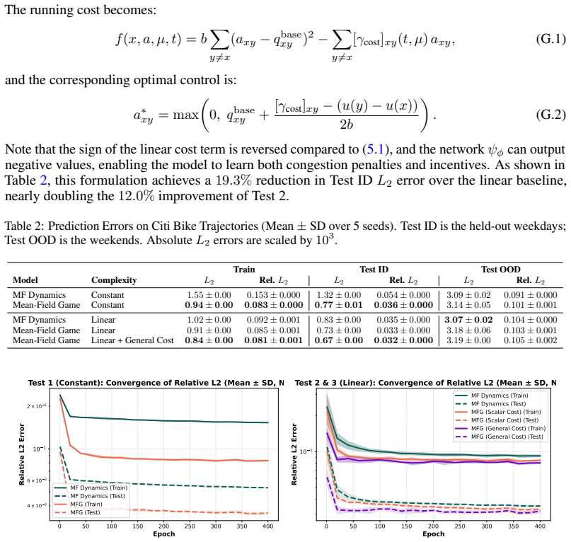
All hyperparameters and instantiations forγ i,min andγ i,max are reported in App
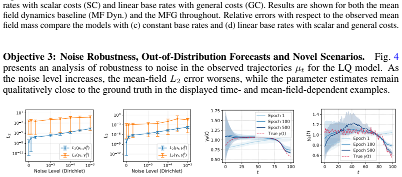
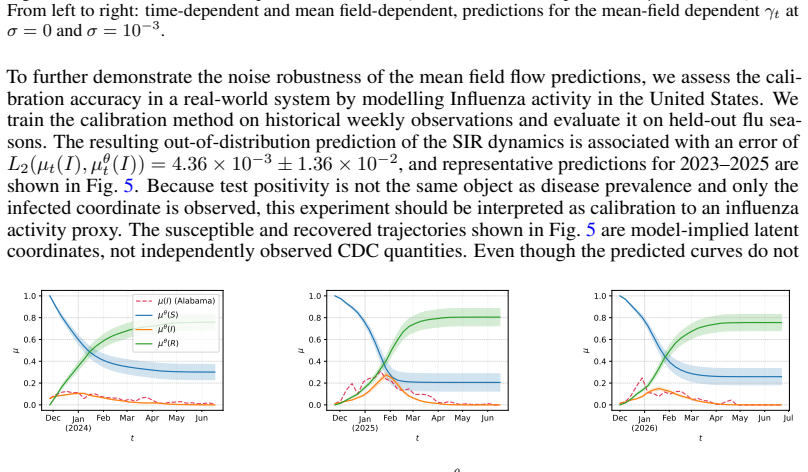
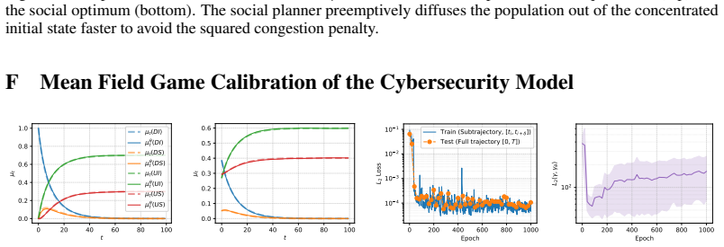
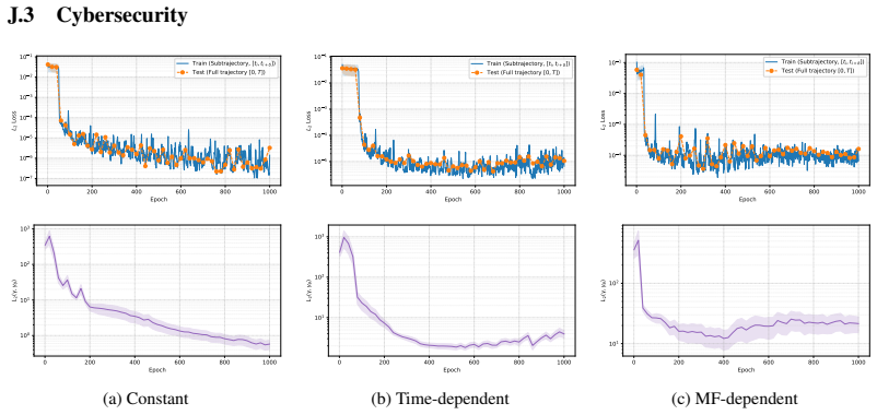
Mean field dependent: γi(t, µ) =γ i,min + (γi,max −γ i,min)µ(0), scaling linearly with the mass in the first state. All hyperparameters and instantiations forγ i,min andγ i,max are reported in App. I. Noise Robustness.We evaluate the robustness of our approach by introducing Dirichlet noise to the observed mean field distributions. Specifically, for a giv...
-
[63]
Forward Equation: The mean field µt satisfies the FPK equation (E.2) with the optimal controlα ∗. 2.Backward Adjoint Equation: The adjoint stateu t satisfies: −∂tut(x) = X y̸=x α∗ t,xy(ut(y)−ut(x))+fγ(t, x, α∗ t , µt)+ X y∈[d] µt(y) ∂fγ ∂µ(x) + ∂fγ ∂γ ∂γ ∂µ(x) , (E.3) where the partial derivatives inside the sum are evaluated at(t, y, α∗ t (y), µt). The t...
-
[64]
This sig- nificantly reduces the natural "free" diffusion of the agents, meaning they remain stationary unless explicitly pushed by the congestion gradients
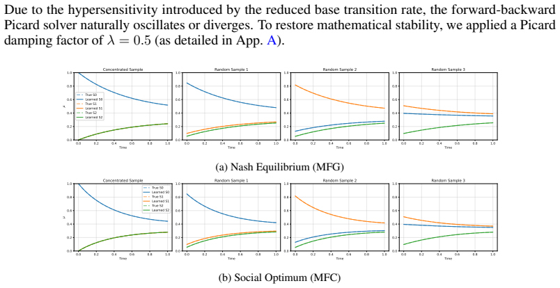
Reduced Base Transition Rate:We lower the base transition rate to axy ≈0.3 . This sig- nificantly reduces the natural "free" diffusion of the agents, meaning they remain stationary unless explicitly pushed by the congestion gradients
-
[65]
systemic risk
Squared Congestion Cost:We adopt a squared congestion penalty cµ(x)2, with c= 2 . By taking the derivative with respect to µ(x), the MFC social planner incurs an additional penalty of 2cµ(x) in the HJB equation. This anticipatory "systemic risk" term strongly forces the planner to evacuate crowded states faster than the selfish MFG agents. 25 Due to the h...
2024
discussion (0)
Sign in with ORCID, Apple, or X to comment. Anyone can read and Pith papers without signing in.