Quantum Renyi relative entropies on a spin chain with interface defects

Ra\'ul Arias

REVIEW 3 major objections 5 minor 32 references

Quantum Renyi relative entropies on a spin chain with interface defects

T0 review · 3 major / 5 minor · reviewed 2026-08-14 · deepseek-v4-flash

Challenge this review Re-run · record.json Download PDF Read on arXiv ↗ Review JSON

Pith's one-line read The Rényi relative entropies of a defect fermion chain obey one closed formula.

desk verdict A competent numerical study of quantum Rényi relative entropies for a defected free-fermion chain, whose advertised 'analytic expression' is really an in-sample curve fit; worth refereeing, but only after the claims are reframed and validated. read the letter →

arxiv 1908.01787 v2 pith:6YWFZZTY submitted 2019-08-05 cond-mat.stat-mech hep-thquant-ph

Raúl Arias This is my paper · ORCID

classification cond-mat.stat-mechhep-thquant-ph

keywords quantumRényirelativeentropyfreefermionchaininterfacedefecteffectivecentralchargefidelitycorrelationmatrixAndersonorthogonalitycatastrophe

verification ladder T0 review T1 audit T2 compute T3 formal

The pith

A machine-rendered reading of the paper's core claim, the machinery that carries it, and where it could break.

The reading

This paper analyzes the quantum Rényi relative entropies between the homogeneous state of an infinite free-fermion chain and the state with an interface defect, for Rényi order α between 1/2 and 1. It claims that, for a subsystem of length L, every such relative entropy is given by a single analytic expression whose only defect dependence enters through the effective central charge of the chain. If true, the whole family of relative entropies, including quantum fidelity at α=1/2 and the relative entropy at α→1, is characterized by just two parameters: the subsystem size and the defect's effective central charge. The paper also finds the same functional dependence for a local potential defect, suggesting a measure of universality across defect types.

What carries the argument

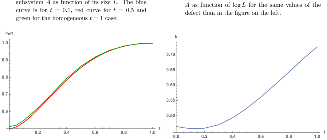
The computation rests on the Gaussian structure of the reduced density matrices: the entanglement Hamiltonian is $H=\log(C^{-1}-1)$ in terms of the correlation matrix $C$, and the Rényi relative entropy can be written directly in terms of the two correlation matrices $C$ and $C'$ (equation (19)). The defect enters through the effective central charge $c_{\rm eff}(t)$ of the inhomogeneous chain, which interpolates between 1/2 for a completely reflecting defect and 1 for the homogeneous chain. The fitted ansatz $S_\alpha=(b_\alpha/3\log L+d_\alpha)(1-(2c_{\rm eff}-1)^{a_\alpha+c_\alpha L^{-1/2}})$ is the bridge that turns the numerics into a closed formula.

What would settle it

Compute $S_\alpha$ for subsystem lengths well beyond 100 (for example $L=10^4$) and for defects very close to $t=1$ or for $\alpha$ outside the interval $[1/2,1]$, then check whether the data still follows equation (21) with the same fixed coefficients $a_\alpha,b_\alpha,c_\alpha,d_\alpha$; any systematic deviation would disprove the claimed closed formula.

Watch

Extended reading notes

Core claim

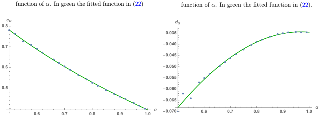
The paper's central result is equation (21): for an interface defect on the boundary of the subsystem, the quantum Rényi relative entropy between the homogeneous reference state and the defected state is $$ S_\$\alpha$(\rho\|\$\sigma$)=\left(\frac{b_\$\alpha$}{3}\log L+d_\$\alpha$\right) \left(1-(2c_{\rm eff}(t)-1)^{a_\$\alpha$+c_\$\alpha$ $L^{{-1/2}}$}\right), $$ where $c_{\rm eff}(t)$ is the effective central charge of the defect, and $a_\alpha,b_\alpha,c_\alpha,d_\alpha$ are fixed polynomial functions of $\alpha$. The same form is reported in section 3.2.2 for a one-site potential defect, with different fitted polynomials for the coefficients. The paper presents numerical evidence that this formula reproduces the data for both types of defects, for $L$ up to 100 and $\alpha$ in the interpolating range from fidelity to relative entropy.

Load-bearing premise

The multiplicative form in equation (21), especially the factor $(1-(2c_{\rm eff}-1)^{a_\alpha+c_\alpha L^{-1/2}})$, is an ansatz chosen by visual inspection of the numerical data and its coefficients are fitted to the same data; nothing in the paper derives this form from first principles.

Editorial extensions

If this is right

The same functional form applies to both a bond defect and a one-site potential defect, so the Rényi relative entropies appear to depend on the defect only through the effective central charge.
At $\alpha=1/2$, the formula gives a fidelity that decays to zero as $L\to\infty$, providing a quantitative version of Anderson's orthogonality catastrophe in this setting.
In the limit $\alpha\to 1$, the formula reduces to the relative entropy and is consistent with the known logarithmic growth of the entanglement entropy difference.
The logarithmic dependence on $L$ with coefficient $b_\alpha/3$ suggests that the relative entropies inherit the central-charge structure of the entanglement entropy.
For defects with the same effective central charge, the formula predicts identical Rényi relative entropies, which could be tested against other lattice realizations.

Reading between the lines

Editorial extensions of the paper, not claims the author makes directly.

A testable extension is to compute $S_\alpha$ for $L$ much larger than 100 and for defects very close to $t=1$; if the $L^{-1/2}$ term in the exponent fails to capture the large-$L$ behavior, the ansatz would need revision.
The polynomial dependence of the coefficients on $\alpha$ suggests that the full family could be derivable from a replica or CFT calculation; if so, the fitted polynomials might be the leading terms of known special functions.
Because the only defect parameter is $c_{\rm eff}$, the Rényi relative entropy itself could serve as an independent numerical estimator of the effective central charge in more complicated inhomogeneous systems.
The author's own conjecture that the result carries over to the transverse Ising chain, via the known correspondence of eigenvalues, is a natural next check that would directly probe the universality of the formula.

Share X Bluesky LinkedIn Reddit HN

Signed reviews

No signed human review yet.

Editorial analysis

A structured set of objections, weighed in public.

Desk editor's note, referee report, and a circularity audit.

Desk Editor's Note

read the letter

You should know this paper has two very different parts. The numerical computation of the Rényi relative entropies via correlator diagonalization, equation (19), is standard and I have no reason to doubt it. That part is solid, and it is genuinely new to have the full QRRE family for a defected free-fermion chain. The packaging of the data into equation (21), with dependence on the effective central charge, is also a new and interesting observation.

The problem is the advertised 'explicit analytic expression'. Equation (21) is not derived. It begins at equation (20) with 'one can try to fit a function on top of the numerical data', and the coefficients a_alpha, b_alpha, c_alpha, d_alpha are fitted to the same S_alpha data that the figures then compare against. The agreement in Figs. 13 and 14 is therefore in-sample self-consistency, not independent confirmation. There are no error bars, no goodness-of-fit statistics, and the L range stops at 100. The abstract's phrase 'explicit analytic expression' overstates what was actually established. The non-polynomial form c_alpha = 2.46172 - 2.06784 alpha^0.3, while the text calls it polynomial, reinforces the sense of shape selection by visual convenience.

That is the load-bearing weakness, and it is real. But it does not sink the paper, because the underlying numerics are believable and the pattern with ceff(t) is worth reporting. The site-defect section is softer still: the gamma coefficients are chosen by inspection, with piecewise regimes in alpha that are not predicted, so that part is closer to a report of numerical observations than to a result with predictive content. The paper would be much stronger if the author reframed (21) explicitly as a numerical fit, gave error bars and a fit-quality measure, and made at least one out-of-sample prediction—say, a larger L or an alpha outside [0.5,1]—to show the form has legs. As written, the central claim is a good hypothesis, not a law.

Who is this for? People working on defect CFT, entanglement measures, and quantum information distances in lattice models. They would find the numerical benchmark useful, and the ceff dependence is suggestive enough that I would want it on the record. I would not cite it as a theorem, but I might cite it as a numerical observation if I worked on that exact model.

For peer review: yes, send it to a serious referee. It is not a desk reject; the computation is competent and the topic is relevant. But the referee should push for the reframing, the error analysis, and an out-of-sample check before acceptance.

Referee Report

3 major / 5 minor

Summary. The paper studies the quantum Rényi relative entropies S_α(ρ||σ) for an infinite free-fermion chain with a boundary defect, where ρ is the defected ground state and σ is the homogeneous one. It uses the Gaussian-state formula (19) to compute S_α numerically from correlation matrices for subsystem sizes up to L=100 and Rényi indices α in [0.5,1). The main proposal is Eq. (21): S_α = (b_α/3 log L + d_α)(1 - (2 c_eff(t) - 1)^{a_α + c_α L^{-1/2}}), with a_α, b_α, c_α, d_α given by the fitted functions in (22). A parallel expression (24) is proposed for an onsite potential defect, with c_eff obtained by numerical interpolation and γ_α(L) given only at α=0.5 and α=0.99. The paper further relates S_{1/2} to fidelity and interprets its L→∞ decay as Anderson orthogonality catastrophe.

Significance. If (21) were a genuine property, it would give a compact one-parameter description of the whole QRRE family in terms of the defect's effective central charge, with immediate limits to fidelity and relative entropy. The numerical method is standard and the paper carefully reproduces known entanglement-entropy results from Peschel. However, the central formula is not derived, and its coefficients are fitted to the same data that are then plotted as agreement; in its present form the paper establishes a numerical fit, not an explicit analytic law. The significance is therefore conditional on further validation or a derivation.

major comments (3)

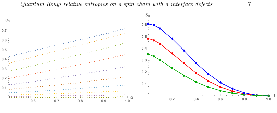
[§3.2.1, Eq. (21)] The central claim is an in-sample fit. Equation (20) is introduced with 'one can try to fit a function on top of the numerical data,' and the four coefficient functions in (22) are adjusted to reproduce the same S_α data against which (21) is checked in Figs. 13–14. No error bars, goodness-of-fit statistics, or held-out data are reported, and the L range ends at L=100. As a result the agreement in Figs. 13–14 is self-consistency of the fit, not independent confirmation. The paper should either derive the functional form (e.g., from the known structure of the entanglement Hamiltonian or from a CFT limit) or validate it out-of-sample (different L, different t, α outside the fitted interval) and quantify the fit quality.
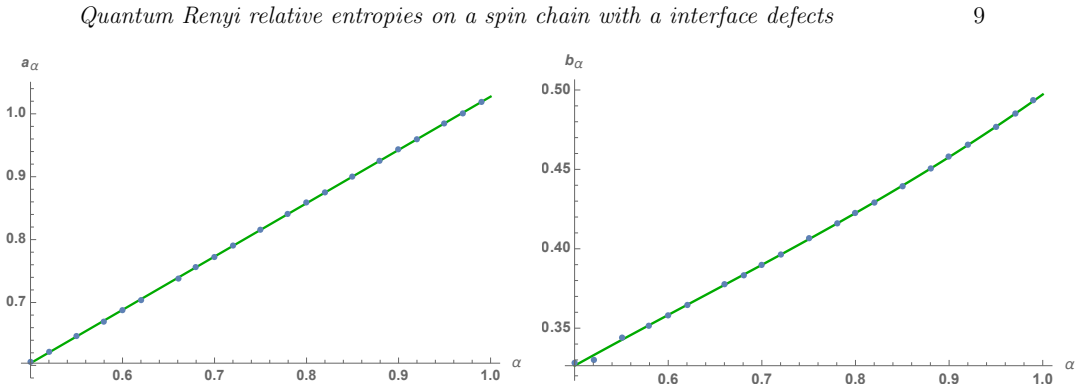
[§3.2.1, Eq. (22)] The text calls the coefficients in (22) polynomial functions, but c_α = 2.46172 − 2.06784 α^{0.3} is not a polynomial. More importantly, the specific shapes (linear a_α, cubic b_α and d_α, α^{0.3} c_α) are chosen by visual inspection with no uncertainty estimates; competing forms (for instance a + c log(L)/L or a + c/L) are not tested. This leaves the claimed dependence on c_eff through the exponent a_α + c_α L^{-1/2} not pinned down. Please report fit uncertainties and test alternative ansätze.
[§3.2.2, Eqs. (24)–(27)] For the onsite defect the paper claims the same dependence on the effective central charge, but c_eff(Δ) is only an interpolating function and no analytic expression is given. The L-dependence of γ_α is described by three different regimes, yet only the endpoint values γ_0.5 = 0.536104 and γ_0.99 = 0.71725 + 0.015165 log L are reported in (27); the intermediate α behavior and the coefficients c_1..c_4 are not given. The agreement claimed in Figs. 17–18 therefore covers only two α values and cannot substantiate the generic claim in (24).

minor comments (5)

[Abstract and Conclusions] The phrase 'explicit analytic expression' overstates the status of (21)–(22), which contain numerically fitted coefficients; please rephrase as a 'numerical expression' or include a clear statement of the fitting procedure and its limitations.
[Throughout] There are several typos and grammatical issues, e.g., 'a interface defects', 'realtive', 'measurementes', 'Coeﬀcient', and 'α⊂ [1/2,1)' should be 'α∈[1/2,1)'.
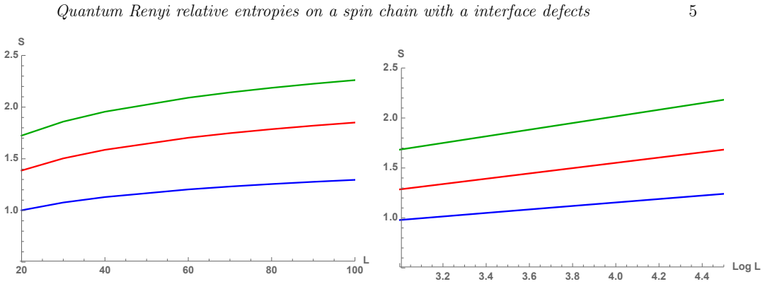
[§3.2.1, Fig. 14] The text says Fig. 14 is for fixed L=80, while the caption says L=100; one of these is incorrect and should be corrected.
[§3.2.1, Eq. (17)] The statement that Δ⟨Hσ⟩ ∼ φ(t) + ϕ(t) log(L) with ranges −0.30008 ≤ φ(t) ≤ 0 and −0.0009 ≤ ϕ(t) ≤ 0 is introduced without derivation or error estimates.
[§3.2.1, Eq. (21)] The numerical exploration is restricted to α in [0.5, 0.99] and L up to 100; please clarify whether (21) is claimed beyond this region or only as an interpolation on the explored domain.

Circularity Check

2 steps flagged · score 7.0 of 10

Equation (21) is an in-sample curve fit, not an independent analytic prediction: the ansatz is chosen by inspection and its coefficients are fitted to the same numerical S_alpha data it is then used to reproduce.

fitted input called prediction [Section 3.2.1, Eq. (20)-(22), Figs. 13-14]
"Then, one can try to fit a function on top of the numerical data which vanishes at t = 1. The proposed function for the α = 0.99 case is S0.99 = β (1− (2ceff (t)− 1)γ). For fixed L and α one can obtain the coefficients β and γ in order to obtain a perfect agreement with the numerical data. ... by studying the coefficients aα,bα,cα,dα as function of α we can arrive to the general formula for the quantum Renyi relative entropies for this problem Sα (ρ||σ) = (bα/3 log(L) + dα)(1− (2ceff(t)−1)^{aα+cαL^{−1/2}}), (21)"

Equation (21) is not derived from Eq. (19); its functional form is chosen by visual inspection and the four coefficient functions in Eq. (22) are fitted to the very same S_alpha(L,t) numerical data that Figs. 13 and 14 then compare against Eq. (21). The agreement is therefore in-sample self-consistency, not independent confirmation. The advertised dependence on ceff(t) is built into the ansatz by construction, and no extrapolation to larger L, different alpha ranges, or other defects is shown.
fitted input called prediction [Section 3.2.2, Eqs. (24)-(27), Figs. 17-18]
"Performing the same analysis than for the previous case we found that Sα(ρ||σ) = ... (24) ... The most interesting are the limiting cases which are related to the fidelity and the relative entropy, in that cases the coefficient γα(L) are γ0.5 = 0.536104, γ0.99 = 0.71725 + 0.015165 log(L). (27) Using these numbers we showed in figures 17 and 18 how the numerical data and the equation (24) agrees perfectly."

The same fitting procedure is repeated for the onsite-potential defect: the coefficients b_alpha, d_alpha and the exponent gamma_alpha(L) are determined by fitting the numerical S_alpha data, with the L-dependence of gamma even split into three empirically chosen regimes. Figures 17 and 18 then plot the fitted formula against the same data points. This establishes internal consistency of the parametrization, not an independent prediction or a derived law.

full rationale

The numerical evaluation of S_alpha via Eq. (19) from diagonalized correlators is self-contained and not circular; Eq. (19) is a known exact representation and is applied directly. The circularity lies in the paper's central claim that an 'explicit analytic expression' for all QRRE has been found. In Section 3.2.1 the paper explicitly says 'one can try to fit a function on top of the numerical data', then fits beta and gamma 'in order to obtain a perfect agreement with the numerical data', then fits the coefficient functions a_alpha, b_alpha, c_alpha, d_alpha in Eq. (22) to the same dataset, and finally displays agreement with those same points. The potential-defect section repeats the identical procedure. Thus Eq. (21) is a compact regression formula, and the agreement plots are in-sample. There is no load-bearing self-citation issue: ceff(t) comes from prior independent work (Ref. [15] and related literature), but using ceff as a variable in an ansatz does not derive the S_alpha law. No out-of-sample checks, error bars, or goodness-of-fit measures are provided, so the non-circular content of the claimed law is limited to the original numerical data itself. Score 7 reflects that the central claim largely reduces to a fit, while the raw numerical computations remain non-circular.

Assumptions & free parameters 8 free parameters · 4 assumptions · 0 invented entities

The central formula is a curve fit, so the coefficient functions are free parameters tuned to numerical data. The physical content is borrowed from the known effective central charge of the defect; no new entities are introduced.

free parameters (8)

a_alpha = 0.847619 alpha + 0.17972 = slope 0.847619, intercept 0.17972
Fit to the numerically determined exponent coefficient a_alpha in (21), over the fitted alpha window.
b_alpha = 0.255266 alpha^3 - 0.481121 alpha^2 + 0.616596 alpha + 0.106444 = cubic polynomial coefficients
Fit to the numerically determined logarithmic prefactor b_alpha in (21).
c_alpha = 2.46172 - 2.06784 alpha^0.3 = 2.46172 and 2.06784, exponent 0.3
Fit to the numerically determined L^(-1/2) coefficient c_alpha in (21).
d_alpha = -0.0232422 alpha^3 - 0.0978656 alpha^2 + 0.254972 alpha - 0.168467 = cubic polynomial coefficients
Fit to the additive constant d_alpha in (21).
site-defect b_alpha = 0.78053 alpha^3 - 1.22826 alpha^2 + 0.999614 alpha - 0.00375985 = cubic polynomial coefficients
Fit to the prefactor in (24) for the onsite defect case.
site-defect d_alpha = 1.51467 alpha^0.8 - 0.230572 = 1.51467 and 0.230572, exponent 0.8
Fit to the additive constant in (24) for the onsite defect case.
site-defect gamma_0.5 = 0.536104 = 0.536104
Constant gamma for alpha = 0.5 in (27), fitted to fidelity data.
site-defect gamma_0.99 = 0.71725 + 0.015165 log(L) = 0.71725 and 0.015165
Logarithmic gamma for alpha = 0.99 in (27), fitted to relative entropy data.

assumptions (4)

standard math Gaussian fermionic states have reduced density matrices of exponential form, with entanglement Hamiltonian H = log(C^(-1) - 1).
Used in equations (2) and (3) of section 2; standard for free fermions but not re-derived.
domain assumption Equation (19) expresses QRRE in terms of correlation matrices of the two states.
Taken from appendix A of reference [14]; this is the computational foundation of the paper and is not derived here.
domain assumption The effective central charge ceff(t) is given by equations (11)-(12) from reference [15].
Borrowed from prior work by Peschel and collaborators; used as the physical input in the ansatz (21).
ad hoc to paper For the onsite defect, an interpolating function for ceff(D) is used instead of an analytic expression.
Section 3.2.2 states no analytic form is available, so an interpolation is introduced; the claim that S_alpha has the same central-charge dependence depends on this choice.

how reviews work

0 comments

Cite this review

Pith. "Pith review of Quantum Renyi relative entropies on a spin chain with interface defects." pith.science (2026). https://pith.science/paper/6YWFZZTY

@misc{pith2026190801787,
  author       = {Pith},
  title        = {Pith review of: Quantum Renyi relative entropies on a spin chain with interface defects},
  year         = {2026},
  howpublished = {\url{https://pith.science/paper/6YWFZZTY}},
  note         = {Machine review of arXiv:1908.01787}
}

read the original abstract

We compute the quantum Renyi relative entropies in an infinite spinless fermionic chain with a defect. Doing a numerical analysis we will show that the resulting quantity depends non trivially on the effective central charge of the theory. Moreover, we will see that an explicit analytic expression can be written for all of them and from that, one can read the quantum fidelity and the relative entropy.

Figures

Figures reproduced from arXiv: 1908.01787 by the authors.

**Figure 1.** Entanglement Entropy of the subsystem A as function of its size L. The blue curve is for t = 0.1, red curve for t = 0.5 and green for the homogeneous t = 1 case. 3.2 3.4 3.6 3.8 4.0 4.2 4.4 Log L 1.0 1.5 2.0 2.5 S [PITH_FULL_IMAGE:figures/full_fig_p005_1.png] view at source ↗

**Figure 3.** Effective central charge as function of t. The red line is the analytic function (11) and the green line the numerical result. 0.0 0.2 0.4 0.6 0.8 1.0 t 0.50 0.55 0.60 0.65 0.70 k [PITH_FULL_IMAGE:figures/full_fig_p005_3.png] view at source ↗

**Figure 6.** Sα(ρ||σ) fot three different values of α and L = 100. In blue the relative entropy, S0.99, in red S0.75 and in green the one related to the fidelity, S0.5 where C is the correlation matrix of the state σ and C 0 is the correlation matrix of state ρ. 3.2. Numerical results In this section we will show that the numerical analysis lead to a closed equation for the quantum Renyi relative entropies. The strategy is diago… view at source ↗

Figures from the paper (6 more)

**Figure 8.** Figure 8: Coefficient γ in equation (21) as function of L. In green the analytic function and the points are the numerical data. see how is the behavior of the coefficients as function of the length. Again for the α = 0.99 case this goes as β(L) = b0.99 3 log L + d0.99, γ(L) = a…

**Figure 9.** Figure 9: Coefficient aα in equation (21) as function of α. In green the fitted function in (22) 0.6 0.7 0.8 0.9 1.0 α 0.35 0.40 0.45 0.50 bα [PITH_FULL_IMAGE:figures/full_fig_p009_9.png]

**Figure 12.** Figure 12: Coefficient dα in equation (21) as function of α. In green the fitted function in (22). this system ∆hHσi ∼ φ(t) + ϕ(t) log(L) where the coefficients φ and ϕ depends on t but they are in the range −0.30008 ≤ φ(t) ≤ 0, −0.0009 ≤ ϕ(t) ≤ 0 when 0 ≤ t ≤ 1. Also note that …

**Figure 14.** Figure 14: The figure shows Sα taken for various values of t and L = 100. The continuous curves are drawn using equation (21) and the points are the numerical data. another states for different values of ∆ = 2 sinh ν between 0 and 10. In reference [15] it was shown that the enta…

**Figure 16.** Figure 16: Coeffcient k in equation (9) as function of ∆. 2 4 6 8 10 Δ 0.5 1.0 1.5 2.0 S0.99 [PITH_FULL_IMAGE:figures/full_fig_p011_16.png]

**Figure 17.** Figure 17: S0.99 as function of ∆. The continuous curve is the analytic result (24) with γ0.99 taken from equation (27), the points are the numerical result. 2 4 6 8 10 Δ 0.2 0.4 0.6 0.8 S0.5 [PITH_FULL_IMAGE:figures/full_fig_p011_17.png]

Discussion (0). Continue with ORCID to comment.

Reference graph

Works this paper leans on

32 extracted references · 10 canonical work pages

[1]

Calabrese and J

P. Calabrese and J. L. Cardy, J. Stat. Mech. 0406 (2004) P06002 doi:10.1088/1742- 5468/2004/06/P06002 [hep-th/0405152]

arXiv 2004
[2]

Casini and M

H. Casini and M. Huerta, J. Phys. A 42 (2009) 504007 doi:10.1088/1751-8113/42/50/504007 [arXiv:0905.2562 [hep-th]]

arXiv 2009
[3]

Vedral, Rev

V. Vedral, Rev. Mod. Phys. 74 (2002) 197 doi:10.1103/RevModPhys.74.197 [quant-ph/0102094]

arXiv 2002
[4]

Lashkari, Phys

N. Lashkari, Phys. Rev. Lett. 113 (2014) 051602 doi:10.1103/PhysRevLett.113.051602 [arXiv:1404.3216 [hep-th]]

arXiv 2014
[5]

Holographic second laws of black hole thermodynamics

A. Bernamonti, F. Galli, R. C. Myers and J. Oppenheim, JHEP 1807 (2018) 111 doi:10.1007/JHEP07(2018)111 [arXiv:1803.03633 [hep-th]]

work page Pith review arXiv 2018
[6]

Gu, Shi-Jian, Int. J. Mod. Phys. B 24, 4371(2010) doi:10.1142/S0217979210056335 [arXiv:0811.3127[quant-ph]]

arXiv 2010
[7]

Zanardi, M

P. Zanardi, M. Cozzini, and P. Giorda, Journal of Statistical Mechanics: Theory and Experiment 2 (Feb., 2007) L02002, doi:10.1088/1742-5468/2007/02/L02002 [arXiv: 0606130[quant-ph]]. Quantum Renyi relative entropies on a spin chain with a interface defects 13

work page doi:10.1088/1742-5468/2007/02/l02002 2007
[8]

Arias, D

R. Arias, D. Blanco, H. Casini and M. Huerta, Phys. Rev. D 95 (2017) no.6, 065005 doi:10.1103/PhysRevD.95.065005 [arXiv:1611.08517 [hep-th]], R. Arias, H. Casini, M. Huerta and D. Pontello, Phys. Rev. D 96 (2017) no.10, 105019 doi:10.1103/PhysRevD.96.105019 [arXiv:1707.05375 [hep-th]]

arXiv 2017

Show all 32 references

[9]

Casini, Class

H. Casini, Class. Quant. Grav. 25 (2008) 205021 doi:10.1088/0264-9381/25/20/205021 [arXiv:0804.2182 [hep-th]]

2008 arXiv
[10]

Y. O. Nakagawa and T. Ugajin, J. Stat. Mech. 1709 (2017) no.9, 093104 doi:10.1088/1742- 5468/aa85c1 [arXiv:1705.07899 [cond-mat.stat-mech]]

2017 arXiv
[11]

Ruggiero and P

P. Ruggiero and P. Calabrese, JHEP 1702 (2017) 039 doi:10.1007/JHEP02(2017)039 [arXiv:1612.00659 [hep-th]]

2017 arXiv
[12]

Murciano, P

S. Murciano, P. Ruggiero and P. Calabrese, J. Stat. Mech. (2019) 034001 doi:10.1088/1742- 5468/ab00ec [arXiv:1810.02287 [cond-mat.stat-mech]]

2019 arXiv
[13]

Lashkari, JHEP 1901 (2019) 059 doi:10.1007/JHEP01(2019)059 [arXiv:1810.09306 [hep-th]]

N. Lashkari, JHEP 1901 (2019) 059 doi:10.1007/JHEP01(2019)059 [arXiv:1810.09306 [hep-th]]

2019 arXiv
[14]

Casini, R

H. Casini, R. Medina, I. Salazar Landea and G. Torroba, JHEP 1809 (2018) 166 doi:10.1007/JHEP09(2018)166 [arXiv:1807.03305 [hep-th]]

2018 arXiv
[15]

Peschel, J

I. Peschel, J. Phys. A: Math. Gen. 38, 4327 (2005); doi:10.1088/0305-4470/38/20/002 [arXiv: 0502034 [cond-mat]]

2005 doi
[16]

Sorensen, M.-S

E.S. Sorensen, M.-S. Chang, N. Laﬂorencie, I. Aﬄeck, J. Stat. Mech.: Th. and Exp. (2007)

2007
[17]

Aﬄeck, N

I. Aﬄeck, N. Laﬂorencie, E.S. Srensen, J. Phys. A: Math. and Th., Vol. 42 (2009)

2009
[18]

Saleur, P

H. Saleur, P. Schmitteckert, R. Vasseur, Phys. Rev. B 88, 085413 (2013)

2013
[19]

Peschel, J

I. Peschel, J. Phys. A 36, L205 (2003) doi:10.1088/0305-4470/36/14/101 [arXiv: 0212631 [cond-mat]]

2003 doi
[20]

Casini, M

H. Casini, M. Huerta and R. C. Myers, JHEP 1105 (2011) 036 doi:10.1007/JHEP05(2011)036 [arXiv:1102.0440 [hep-th]]

2011 arXiv
[21]

Cardy and E

J. Cardy and E. Tonni, J. Stat. Mech. 1612 (2016) no.12, 123103 doi:10.1088/1742- 5468/2016/12/123103 [arXiv:1608.01283 [cond-mat.stat-mech]]

2016 arXiv
[22]

Di Giulio, R

G. Di Giulio, R. Arias and E. Tonni, arXiv:1905.01144 [cond-mat.stat-mech]

1905 arXiv
[23]

Eisler, I

V. Eisler, I. Peschel Ann. Phys. (Berlin) 522, 679 (2010). doi:10.1002/andp.201000055 [arXiv:1005.2144 [cond-mat]]

2010 arXiv
[24]

Peschel, V.Eisler J

I. Peschel, V.Eisler J. Phys. A: Math. Theor. 45 (2012) 155301 doi:10.1088/1751-8113/45/15/155301 [arXiv: 1201.4104 [cond-mat]]

2012 arXiv
[25]

Calabrese, M

P. Calabrese, M. Mintchev and E. Vicari, J. Phys. A 45 (2012) 105206 doi:10.1088/1751- 8113/45/10/105206 [arXiv:1110.5713 [cond-mat.stat-mech]]

2012 arXiv
[26]

Muller-Lennert, F

M. Muller-Lennert, F. Dupuis, O. Szehr, S. Fehr, and M. Tomamichel, Journal of Mathematical Physics 54 no. 12, (2013) 122203 doi:10.1063/1.4838856 [arXiv: 1306.3142 [quant-ph]]

2013 arXiv
[27]

M. M. Wilde, A. Winter, and D. Yang, Communications in Mathematical Physics 331 no. 2, (2014) 593622 doi:10.1007/s00220-014-2122-x [arXiv: 1306.1586 [quant-ph]]

2014 arXiv
[28]

Uhlmann, Reports on Mathematical Physics 9 no

A. Uhlmann, Reports on Mathematical Physics 9 no. 2, (1976) 273279 doi:10.1016/0034- 4877(76)90060-4

1976 doi
[29]

Eisler, I

V. Eisler, I. Peschel J. Stat. Mech. (2007) P06005. doi:10.1088/1742-5468/2007/06/P06005 [arXiv:0703379[cond-mat]]

2007 doi
[30]

Anderson, Phys

P. Anderson, Phys. Rev. Lett. 18 (1967), 1049 doi:10.1103/PhysRevLett.18.1049

1967 doi
[31]

Igloi, R

F. Igloi, R. Juhasz, Europhys. Lett. 81, 57003 (2008) doi:10.1209/0295-5075/81/57003 [arXiv: 0709.3927 [cond-mat]]

2008 arXiv
[32]

Igloi, S

F. Igloi, S. Zsolt; Y. Lin, Phys. Rev. B 80, 024405 (2009) doi:10.1103/PhysRevB.80.024405 [arXiv: 0903.3740 [cond-mat]]

2009 arXiv

Pith tools

Reviewed August 14, 2026 · model on record in the stance chip above.

[1] [1]

Calabrese and J

P. Calabrese and J. L. Cardy, J. Stat. Mech. 0406 (2004) P06002 doi:10.1088/1742- 5468/2004/06/P06002 [hep-th/0405152]

arXiv 2004

[2] [2]

Casini and M

H. Casini and M. Huerta, J. Phys. A 42 (2009) 504007 doi:10.1088/1751-8113/42/50/504007 [arXiv:0905.2562 [hep-th]]

arXiv 2009

[3] [3]

Vedral, Rev

V. Vedral, Rev. Mod. Phys. 74 (2002) 197 doi:10.1103/RevModPhys.74.197 [quant-ph/0102094]

arXiv 2002

[4] [4]

Lashkari, Phys

N. Lashkari, Phys. Rev. Lett. 113 (2014) 051602 doi:10.1103/PhysRevLett.113.051602 [arXiv:1404.3216 [hep-th]]

arXiv 2014

[5] [5]

Holographic second laws of black hole thermodynamics

A. Bernamonti, F. Galli, R. C. Myers and J. Oppenheim, JHEP 1807 (2018) 111 doi:10.1007/JHEP07(2018)111 [arXiv:1803.03633 [hep-th]]

work page Pith review arXiv 2018

[6] [6]

Gu, Shi-Jian, Int. J. Mod. Phys. B 24, 4371(2010) doi:10.1142/S0217979210056335 [arXiv:0811.3127[quant-ph]]

arXiv 2010

[7] [7]

Zanardi, M

P. Zanardi, M. Cozzini, and P. Giorda, Journal of Statistical Mechanics: Theory and Experiment 2 (Feb., 2007) L02002, doi:10.1088/1742-5468/2007/02/L02002 [arXiv: 0606130[quant-ph]]. Quantum Renyi relative entropies on a spin chain with a interface defects 13

work page doi:10.1088/1742-5468/2007/02/l02002 2007

[8] [8]

Arias, D

R. Arias, D. Blanco, H. Casini and M. Huerta, Phys. Rev. D 95 (2017) no.6, 065005 doi:10.1103/PhysRevD.95.065005 [arXiv:1611.08517 [hep-th]], R. Arias, H. Casini, M. Huerta and D. Pontello, Phys. Rev. D 96 (2017) no.10, 105019 doi:10.1103/PhysRevD.96.105019 [arXiv:1707.05375 [hep-th]]

arXiv 2017