REVIEW 2 major objections 6 minor 83 references
Quasiperiodic quantum heat engines with a mobility edge
T0 review · 2 major / 6 minor · reviewed 2026-08-14 · deepseek-v4-flash
Pith's one-line read The mobility edge of a quasiperiodic 1D wire acts as a tunable energy filter that yields thermoelectric figures of merit up to ZT ≈ 60.
desk verdict A solid proof-of-principle that a 1D quasiperiodic mobility edge can act as a thermoelectric energy filter, but the headline ZT numbers and the 'orders of magnitude' claim outrun the evidence as presented. read the letter →
The pith
A machine-rendered reading of the paper's core claim, the machinery that carries it, and where it could break.
The reading
What carries the argument
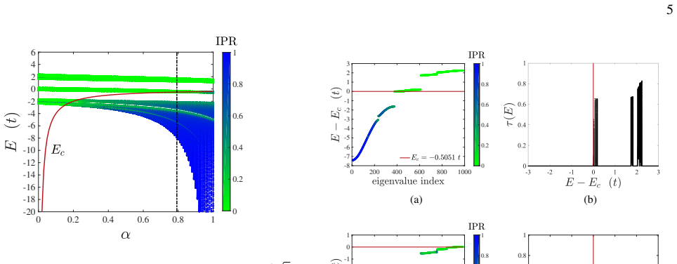
The load-bearing object is the mobility edge $E_c = (1/[\alpha\,\mathrm{sign}(\lambda)])(|t|-|\lambda|)$ of the GAAH model. It splits the single-particle spectrum into localized states below $E_c$ and extended, ballistic states above, making the transmission function $\tau(E) = \gamma^2/|\det[M(E)]|^2$ strongly energy-asymmetric. That asymmetry breaks the particle-hole symmetry of the Fermi-Dirac transport window, so the Seebeck coefficient $S = (1/eT)(\int dE\,(E-\mu)\,\tau(E)[-f'(E)] / \int dE\,\tau(E)[-f'(E)])$ is nonzero and large near the edge. The paper shows that only the coarse-grained profile of the conducting bands, not their fractal fine structure, controls the ratio quantities $S$, $ZT$, and $\eta$, which is why a boxcar approximation to $\tau(E)$ reproduces the thermodynamic performance.
What would settle it
Take a GAAH chain of 987 sites at $T = 0.1\, t/k_B$, fix one phase $\varphi$ instead of averaging over 40 phases, and compute $ZT(\mu)$ around the first two ballistic bands; if the peaks near $ZT \approx 60$ and $ZT \approx 40$ shift or vanish under phase sampling, the single-device prediction fails.
Extended reading notes
Core claim
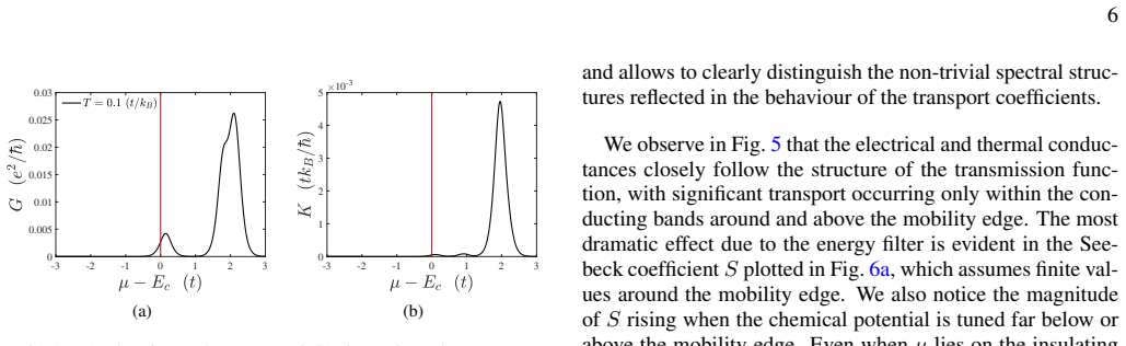
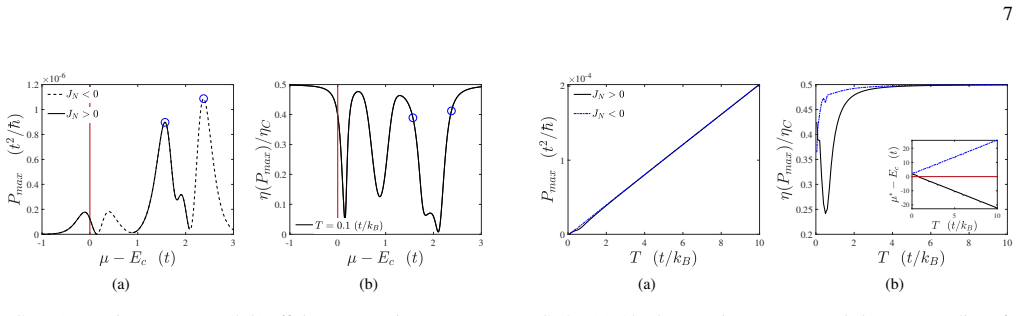
The central claim is that the mobility edge of the generalized Aubry-André-Harper (GAAH) model is an exceptionally effective energy filter for steady-state thermoelectric conversion. The model is a tight-binding chain with on-site potential $V_i = 2\lambda \cos(2\pi b i + \varphi)/[1-\alpha \cos(2\pi b i + \varphi)]$ and an analytically known mobility edge $E_c = (1/[\alpha\,\mathrm{sign}(\lambda)])(|t|-|\lambda|)$. Eigenstates below $E_c$ are localized, so they do not conduct; states above it are extended and ballistic. The resulting transmission function is strongly asymmetric, breaking the particle-hole symmetry that would otherwise cancel the thermoelectric current. Computing the Onsager coefficients through the Landauer-Büttiker formula, the paper finds $ZT \approx 10$ just above the mobility edge, $ZT \approx 60$ and $ZT \approx 40$ at the edges of the first two ballistic bands, and an efficiency at maximum power of $\eta \approx 0.4\,\eta_C$ at $T = 0.1\, t/k_B$. The authors argue the effect is generic: a boxcar-shaped transmission with the same coarse features reproduces the ratio quantities, so any quasiperiodic system with a mobility edge separating ballistic and localized states should behave similarly.
Load-bearing premise
The quantitative results treat the phase-averaged transport coefficients as the behavior of a single physical wire, although the fractal spectrum of the quasiperiodic potential can make individual realizations differ strongly.
Editorial extensions
If this is right
- Linear-response thermoelectric figures of merit of order 10–60 become available in a single non-interacting one-dimensional chain, far above bulk values around $ZT \approx 1$.
- Tuning $\alpha$ and $\lambda$ moves the mobility edge according to $E_c = (1/[\alpha\,\mathrm{sign}(\lambda)])(|t|-|\lambda|)$, so one wire can be reconfigured between high-power and high-efficiency operating points.
- Because the fractal fine structure of the transmission function is irrelevant to $ZT$ and $\eta$, the prediction should carry over to other quasiperiodic systems with a mobility edge and to experimentally realized versions with beyond-nearest-neighbour hopping.
- The proposed platform is testable with ultracold neutral atoms in bichromatic optical lattices, where two-terminal transport measurements are available.
Reading between the lines
- The paper does not report the spread of $ZT$ across the 40 phase values it averages over; measuring that spread for a fixed wire is the natural next step and would show whether a single realization can actually deliver $ZT \approx 60$.
- If the boxcar argument generalizes, the design principle is broader than quasiperiodic systems: any transmission profile with sharp conducting windows separated by gaps could be engineered into a high-$ZT$ thermoelectric, for instance in superlattices or nanostructured wires.
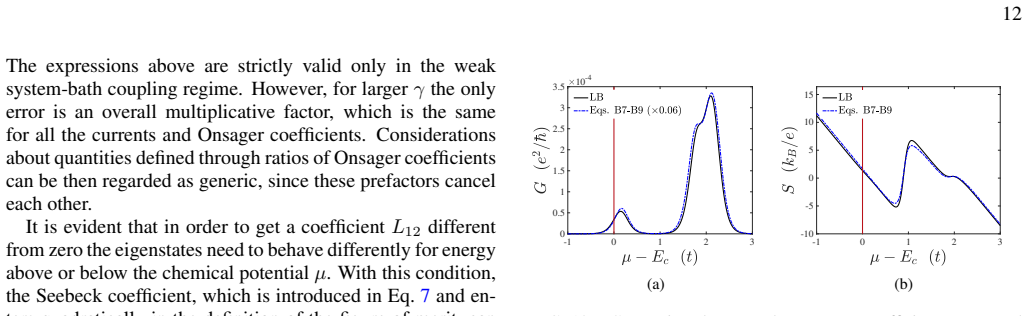
- Because the ratio quantities are independent of the system-bath coupling $\gamma$ while power grows up to an optimal $\gamma$, experimental implementations could maximize power by tuning the coupling without sacrificing efficiency.
- The linear-response $ZT$ values may not persist under large temperature biases; extending the calculations beyond linear response would reveal whether the mobility-edge filter remains advantageous in the strongly driven regime.
Signed reviews
Editorial analysis
A structured set of objections, weighed in public.
Referee Report
Summary. The manuscript proposes a steady-state thermoelectric heat engine based on the generalized Aubry-André-Harper (GAAH) model, whose single-particle mobility edge can be tuned by potential parameters. Using non-equilibrium Green's function and Landauer-Büttiker calculations for a 987-site chain with γ = t, the authors compute the Onsager coefficients for one parameter set (α = 0.792, λ = -0.8t), average over 40 quasiperiodic phases, and report low-temperature figures of merit ZT ≈ 10 near the mobility edge and ZT ≈ 60 and ≈ 40 at the edges of the first two ballistic bands, with efficiency at maximum power up to about 0.4η_C. They further compare with a clean wire and with a boxcar approximation to argue that the qualitative behavior is generic for 1D quasiperiodic systems with a mobility edge.
Significance. If the quantitative results are robust, this would be a notable contribution: it identifies a concrete, experimentally relevant 1D system in which a mobility edge acts as a tunable energy filter, and it opens a new application of quasiperiodic systems in quantum thermodynamics. The work is built on standard and internally consistent NEGF transport theory; the comparison against a clean wire and a boxcar transmission function is a useful sanity check; and the use of the exact analytic mobility-edge expression of Ref. [34] makes the energy-filter interpretation transparent. The main limitations are that the headline quantitative figures are obtained from phase-averaged transport coefficients without statistical or finite-size validation, and the 'several orders of magnitude' claim in the abstract is not substantiated by any explicit comparison to prior predictions.
major comments (2)
- [Sec. IV A and Fig. 6] The statement 'All quantities shown in this section are obtained numerically and averaged over the phase φ' is not sufficient support for the headline values ZT ≈ 60 and ZT ≈ 40. ZT is a nonlinear function of the Onsager coefficients (ZT = L12^2/det L), so computing it from phase-averaged L_ij yields an ensemble quantity that need not describe any single fixed-phase device. In a finite incommensurate chain the spectrum and transmission are strongly φ-dependent, especially at band edges where the ZT peaks occur. As written, the paper provides no variance, no phase-resolved histogram, and no finite-size scaling (only N = 987 is used). Please provide phase-resolved distributions of ZT and η at the peak positions, or alternatively present a convincing self-averaging argument, and report results for at least two other system sizes. Without this, the quantitative predictions in Figs. 6 and 7 cannot be distinguished from phase-averaging artifacts.
- [Abstract and Sec. I] The abstract claims that the effects 'exceeding existing predictions by several orders of magnitude' is not supported by the manuscript. No specific prior prediction is cited and compared; the only quantitative baseline in the paper is the clean-wire calculation of Sec. IV D, which is not an 'existing prediction' from the literature. Please either cite and compare against specific earlier thermoelectric predictions or reformulate the abstract to state the actual comparison made, for instance by comparing directly with the clean-wire and AAH-model results obtained in the paper. In its current form the claim is too vague to be checked.
minor comments (6)
- [Abstract] The name 'Aubrey-André-Harper' should be 'Aubry-André-Harper'.
- [Sec. II C, Eq. (10)] The text says the particles are 'spinless electrons', but the Landauer integrals include a factor 2 'due to spin degeneracy'. This is internally inconsistent; if the model is spinless the factor should be 1, while if the factor 2 is retained the model is spin-degenerate. The inconsistency does not affect S, ZT, or η because the factor cancels in ratios, but it should be fixed.
- [Sec. II A, after Eq. (16)] The sentence 'the last site of the system is coupled to the right lead (denoted by the subscript L)' should say 'denoted by the subscript R'.
- [Fig. 4 caption] The caption says '(b)-(d) The transmission functions associated respectively to the first and second configuration', but panels (c) is a spectrum and only (b) and (d) are transmission functions. Please rephrase to ' (b) and (d) Transmission functions ...'.
- [Sec. IV A] The decision to focus on a single representative parameter set is reasonable for a first study, but the abstract's word 'versatile' would be better supported by at least one additional parameter set with thermoelectric results; Fig. 4(c)-(d) provides a second spectrum and transmission but no corresponding transport coefficients or ZT.
- [Appendix A] The claim that 'the forms of L11, L12 and L22 ... remain the same regardless of γ, up to an overall factor' is supported in Fig. 11 only for L11 and for the ratio ZT. Showing the analogous curves for L12 and L22 would make the γ-independence argument more complete.
Circularity Check
No significant circularity: the thermoelectric predictions follow from an exact numerical solution of the stated GAAH Hamiltonian with no fitted parameters in the central results.
full rationale
The paper's central results (ZT and efficiency at maximum power) are computed from the microscopic GAAH Hamiltonian via the NEGF transmission function and Landauer-Büttiker integrals. Eq. (20) gives tau(E) = gamma^2 |G_1N(E)|^2 directly from the Hamiltonian and the wide-band self-energies, with no adjustable parameters. The Onsager coefficients are then obtained from Eq. (12), and ZT and eta(Pmax) from Eqs. (8) and (9). The only input from outside the derivation is the analytical mobility-edge expression Eq. (22), which is attributed to Ref. [34] (Ganeshan et al.), an external group, and is independently consistent with the paper's IPR data in Fig. 3. The self-citations (Refs. [51–56]) are used to contextualize prior transport characterization and to justify the weak-coupling expressions of Appendix B; they do not set the values of ZT or efficiency, and the Appendix B proportionality constants cancel in the dimensionless ratios that are actually reported. Section IV E's boxcar model is a post-hoc consistency check, not the source of the headline numbers. The phase-averaging procedure (Sec. IV A) is a robustness concern about whether a single device reproduces the ensemble-averaged ZT, but that is a question of statistical representativeness, not circularity: no prediction is defined in terms of the quantity it is said to explain. Accordingly, no circular step is exhibited.
Assumptions & free parameters
free parameters (4)
- alpha (GAAH potential deformation) =
0.792
- lambda (GAAH potential strength) =
-0.8 t
- Proportionality factor for weak-coupling Onsager comparison =
0.06
- Proportionality factor for boxcar approximation =
6.0
assumptions (7)
- domain assumption Landauer-Büttiker formalism with wide-band limit (energy-independent coupling γ) describes coherent transport in the GAAH wire
- domain assumption The mobility edge formula Ec = (1/(α sign λ))(|t| − |λ|) from Ref. [34] is exact and applies to the finite N=987 open system with γ=t
- ad hoc to paper Phase-averaged transport coefficients (40 values of φ) are representative of a single device
- ad hoc to paper The boxcar transmission function captures the essential physics of any quasiperiodic system with a mobility edge
- domain assumption Eigenstate scaling for localized states: Φ^2 ~ e^{-N} for n<n* and Φ^2 ~ 1/N for n>n*
- ad hoc to paper Eigenfunctions contribute approximately equal weight for each n>n* in the Onsager sums
- domain assumption Linear response and time-reversal symmetry (Onsager relation L12=L21) hold
Cite this review
Pith. "Pith review of Quasiperiodic quantum heat engines with a mobility edge." pith.science (2026). https://pith.science/paper/2C3ZVYFB
@misc{pith2026190805139,
  author       = {Pith},
  title        = {Pith review of: Quasiperiodic quantum heat engines with a mobility edge},
  year         = {2026},
  howpublished = {\url{https://pith.science/paper/2C3ZVYFB}},
  note         = {Machine review of arXiv:1908.05139}
}
read the original abstract
Steady-state thermoelectric machines convert heat into work by driving a thermally-generated charge current against a voltage gradient. In this work, we propose a new class of steady-state heat engines operating in the quantum regime, where a quasi-periodic tight-binding model that features a mobility edge forms the working medium. In particular, we focus on a generalization of the paradigmatic Aubrey-Andr\'e-Harper (AAH) model, known to display a single-particle mobility edge that separates the energy spectrum into regions of completely delocalized and localized eigenstates. Remarkably, these two regions can be exploited in the context of steady-state heat engines as they correspond to ballistic and insulating transport regimes. This model also presents the advantage that the position of the mobility edge can be controlled via a single parameter in the Hamiltonian. We exploit this highly tunable energy filter, along with the peculiar spectral structure of quasiperiodic systems, to demonstrate large thermoelectric effects, exceeding existing predictions by several orders of magnitude. This opens the route to a new class of highly efficient and versatile quasi-periodic steady-state heat engines, with a possible implementation using ultracold neutral atoms in bichromatic optical lattices.
Figures


Figures from the paper (10 more)





Reference graph
Works this paper leans on
-
[34]
Ganeshan, J
S. Ganeshan, J. H. Pixley, and S. Das Sarma, Phys. Rev. Lett. 114, 146601 (2015)
2015
-
[1]
Kosloff and A
R. Kosloff and A. Levy, Annu. Rev. Phys. Chem. 65, 365 (2014)
2014
-
[2]
M. T. Mitchison, Contemp. Phys. (2019), 10.1080/00107514.2019.1631555
arXiv 2019
-
[3]
M. O. Scully, K. R. Chapin, K. E. Dorfman, M. B. Kim, and A. Svidzinsky, Proc. Nat. Acad. Sci. 108, 15097 (2011)
2011
-
[4]
Brunner, M
N. Brunner, M. Huber, N. Linden, S. Popescu, R. Silva, and P. Skrzypczyk, Phys. Rev. E89, 032115 (2014)
2014
-
[5]
L. A. Correa, J. P. Palao, D. Alonso, and G. Adesso, Sci. Rep. 4, 3949 (2014)
work page 2014
-
[6]
N. Killoran, S. F. Huelga, and M. B. Plenio, J. Chem. Phys. 143, 155102 (2015)
work page 2015
- [7]
Show all 83 references
-
[8]
Ghosh, C
A. Ghosh, C. L. Latune, L. Davidovich, and G. Kurizki, Proc. Nat. Acad. Sci. 114, 12156 (2017)
2017
-
[9]
Yunger Halpern, C
N. Yunger Halpern, C. D. White, S. Gopalakrishnan, and G. Refael, Phys. Rev. B 99, 024203 (2019)
2019
-
[10]
Klatzow, J
J. Klatzow, J. N. Becker, P. M. Ledingham, C. Weinzetl, K. T. Kaczmarek, D. J. Saunders, J. Nunn, I. A. Walmsley, R. Uzdin, and E. Poem, Phys. Rev. Lett. 122, 110601 (2019)
2019
-
[11]
Benenti, G
G. Benenti, G. Casati, K. Saito, and R. S. Whitney, Phys. Rep. 694, 1 (2017)
2017
-
[12]
Josefsson, A
M. Josefsson, A. Svilans, A. Burke, E. A. Hoffmann, S. Fahlvik, C. Thelander, M. Leijnse, and H. Linke, Nat. Nan- otechnol. 13 (2018)
2018
-
[13]
Giazotto, J
F. Giazotto, J. W. A. Robinson, J. S. Moodera, and F. S. Berg- eret, Appl. Phys. Lett. 105, 062602 (2014)
2014
-
[14]
Zebarjadi, K
M. Zebarjadi, K. Esfarjani, M. S. Dresselhaus, Z. F. Ren, and G. Chen, Energy Environ. Sci. 5, 5147 (2012)
2012
-
[15]
L. E. Bell, Science 321, 1457 (2008)
2008
-
[16]
Dresselhaus, G
M. Dresselhaus, G. Chen, M. Tang, R. Yang, H. Lee, D. Wang, Z. Ren, J.-P. Fleurial, and P. Gogna, Adv. Mater. 19, 1043 (2007)
2007
-
[17]
Mani and C
A. Mani and C. Benjamin, Phys. Rev. E 96, 032118 (2017)
2017
-
[18]
G. D. Mahan and J. O. Sofo, Proc. Natl. Acad. Sci 93, 7436 (1996)
1996
-
[19]
Whitney, Phys
R. Whitney, Phys. Rev. Lett. 112, 130601 (2014)
2014
-
[20]
Bosisio, C
R. Bosisio, C. Gorini, G. Fleury, and J.-L. Pichard, New Jour- nal of Physics 16, 095005 (2014)
2014
-
[21]
P. W. Anderson, Phys. Rev. 109, 1492 (1958)
1958
-
[22]
Semeghini, M
G. Semeghini, M. Landini, P. Castilho, S. Roy, G. Spagnolli, A. Trenkwalder, M. Fattori, M. Inguscio, and G. Modugno, Nat. Phys. 11, 554 EP (2015). 10
2015
-
[23]
Sivan and Y
U. Sivan and Y . Imry, Phys. Rev. B33, 551 (1986)
1986
-
[24]
Yamamoto, A
K. Yamamoto, A. Aharony, O. Entin-Wohlman, and N. Hatano, Phys. Rev. B 96, 155201 (2017)
2017
-
[25]
Abrahams, P
E. Abrahams, P. W. Anderson, D. C. Licciardello, and T. V . Ramakrishnan, Phys. Rev. Lett. 42, 673 (1979)
1979
-
[26]
Aubry and G
S. Aubry and G. Andr ´e, Ann. Israel Phys. Soc 3, 18 (1980)
1980
-
[27]
P. G. Harper, Proc. Phys. Soc. Sec. A 68, 874 (1955)
1955
-
[28]
Ostlund, R
S. Ostlund, R. Pandit, D. Rand, H. J. Schellnhuber, and E. D. Siggia, Phys. Rev. Lett. 50, 1873 (1983)
1983
-
[29]
Kohmoto, B
M. Kohmoto, B. Sutherland, and C. Tang, Phys. Rev. B 35, 1020 (1987)
1987
-
[30]
Last, Commun
Y . Last, Commun. Math. Phys.164, 421 (1994)
1994
-
[31]
Hiramoto and M
H. Hiramoto and M. Kohmoto, Int. J. Mod. Phys. B 06, 281 (1992)
1992
-
[32]
Rossignolo and L
M. Rossignolo and L. Dell’Anna, Phys. Rev. B 99, 054211 (2019)
2019
-
[33]
X. Li, X. Li, and S. Das Sarma, Phys. Rev. B 96, 085119 (2017)
2017
-
[35]
Biddle, D
J. Biddle, D. J. Priour, B. Wang, and S. Das Sarma, Phys. Rev. B 83, 075105 (2011)
2011
-
[36]
Biddle and S
J. Biddle and S. Das Sarma, Phys. Rev. Lett. 104, 070601 (2010)
2010
-
[37]
Biddle, B
J. Biddle, B. Wang, D. J. Priour, and S. Das Sarma, Phys. Rev. A 80, 021603 (2009)
2009
-
[38]
D. J. Boers, B. Goedeke, D. Hinrichs, and M. Holthaus, Phys. Rev. A 75, 063404 (2007)
2007
-
[39]
Das Sarma, S
S. Das Sarma, S. He, and X. C. Xie, Phys. Rev. B 41, 5544 (1990)
1990
-
[40]
Das Sarma, S
S. Das Sarma, S. He, and X. C. Xie, Phys. Rev. Lett. 61, 2144 (1988)
1988
-
[41]
Settino, N
J. Settino, N. Lo Gullo, A. Sindona, J. Goold, and F. Plastina, Phys. Rev. A 95, 033605 (2017)
2017
-
[42]
Roati, C
G. Roati, C. D’Errico, L. Fallani, M. Fattori, C. Fort, M. Za- ccanti, G. Modugno, M. Modugno, and M. Inguscio, Nature 453, 895 (2008)
2008
-
[43]
Schreiber, S
M. Schreiber, S. S. Hodgman, P. Bordia, H. P. L ¨uschen, M. H. Fischer, R. V osk, E. Altman, U. Schneider, and I. Bloch, Sci- ence 349, 842 (2015)
2015
-
[44]
H. P. L ¨uschen, P. Bordia, S. S. Hodgman, M. Schreiber, S. Sarkar, A. J. Daley, M. H. Fischer, E. Altman, I. Bloch, and U. Schneider, Phys. Rev. X7, 011034 (2017)
2017
-
[45]
H. P. L ¨uschen, S. Scherg, T. Kohlert, M. Schreiber, P. Bordia, X. Li, S. Das Sarma, and I. Bloch, Phys. Rev. Lett.120, 160404 (2018)
2018
-
[46]
Kohlert, S
T. Kohlert, S. Scherg, X. Li, H. P. L ¨uschen, S. Das Sarma, I. Bloch, and M. Aidelsburger, Phys. Rev. Lett. 122, 170403 (2019)
2019
-
[47]
X. Li, S. Ganeshan, J. H. Pixley, and S. Das Sarma, Phys. Rev. Lett. 115, 186601 (2015)
2015
-
[48]
Modak and S
R. Modak and S. Mukerjee, Phys. Rev. Lett. 115, 230401 (2015)
2015
-
[49]
Nag and A
S. Nag and A. Garg, Phys. Rev. B 96, 060203 (2017)
2017
-
[50]
Y .-T. Hsu, X. Li, D.-L. Deng, and S. Das Sarma, Phys. Rev. Lett. 121, 245701 (2018)
2018
-
[51]
Purkayastha, J
A. Purkayastha, J. Stat. Mech.: Theory Exp. 2019, 043101 (2019)
2019
-
[52]
Purkayastha, S
A. Purkayastha, S. Sanyal, A. Dhar, and M. Kulkarni, Phys. Rev. B 97, 174206 (2018)
2018
-
[53]
Purkayastha, A
A. Purkayastha, A. Dhar, and M. Kulkarni, Phys. Rev. B 96, 180204 (2017)
2017
-
[54]
V . K. Varma, C. de Mulatier, and M. ˇZnidariˇc, Phys. Rev. E96, 032130 (2017)
2017
- [55]
-
[56]
Balachandran, S
V . Balachandran, S. R. Clark, J. Goold, and D. Poletti, Phys. Rev. Lett. 123, 020603 (2019)
2019
-
[57]
Lebrat, P
M. Lebrat, P. Gri ˇsins, D. Husmann, S. H ¨ausler, L. Corman, T. Giamarchi, J.-P. Brantut, and T. Esslinger, Phys. Rev. X 8, 011053 (2018)
2018
-
[58]
Krinner, T
S. Krinner, T. Esslinger, and J.-P. Brantut, J. Phys. Condens. Matter 29, 343003 (2017)
2017
-
[59]
Kan ´asz-Nagy, L
M. Kan ´asz-Nagy, L. Glazman, T. Esslinger, and E. A. Demler, Phys. Rev. Lett. 117, 255302 (2016)
2016
-
[60]
Krinner, D
S. Krinner, D. Stadler, D. Husmann, J.-P. Brantut, and T. Esslinger, Nature 517, 64 (2014)
2014
-
[61]
Brantut, C
J.-P. Brantut, C. Grenier, J. Meineke, D. Stadler, S. Krinner, C. Kollath, T. Esslinger, and A. Georges, Science 342, 713 (2013)
2013
-
[62]
X. Li, J. H. Pixley, D.-L. Deng, S. Ganeshan, and S. Das Sarma, Phys. Rev. B 93, 184204 (2016)
2016
-
[63]
D.-L. Deng, S. Ganeshan, X. Li, R. Modak, S. Mukerjee, and J. H. Pixley, Ann. Phys. (Berl.) 529, 1600399 (2017)
2017
-
[64]
H. B. Callen, Thermodynamics and an Introduction to Thermo- statistics, (Wiley, New York, 1985)
1985
-
[65]
Yamamoto and N
K. Yamamoto and N. Hatano, Phys. Rev. E 92 (2015)
2015
-
[66]
G. J. Snyder and E. S. Toberer, Nat. Mater. 7, 105 EP (2008)
2008
-
[67]
Shakouri, Annu
A. Shakouri, Annu. Rev. Mater. Res. 41, 399 (2011)
2011
-
[68]
Dubi and M
Y . Dubi and M. Di Ventra, Rev. Mod. Phys.83, 131 (2011)
2011
-
[69]
van Houten, L
H. van Houten, L. W. Molenkamp, C. W. J. Beenakker, and C. T. Foxon, Semicond. Sci. Technol.7, B215 (1992)
1992
-
[70]
S. R. De Groot and P. Mazur,Non-equilibrium thermodynamics (Courier Corporation, 2013)
2013
-
[71]
Onsager, Phys
L. Onsager, Phys. Rev. 37, 405 (1931)
1931
-
[72]
H. J. Goldsmid, Introduction to thermoelectricity , V ol. 121 (Springer, 2010)
2010
-
[73]
Van den Broeck, Phys
C. Van den Broeck, Phys. Rev. Lett. 95, 190602 (2005)
2005
-
[74]
F. L. Curzon and B. Ahlborn, Am. J. Phys. 43, 22 (1975)
1975
-
[75]
Z. Bian, M. Zebarjadi, R. Singh, Y . Ezzahri, A. Shakouri, G. Zeng, J.-H. Bahk, J. E. Bowers, J. M. O. Zide, and A. C. Gossard, Phys. Rev. B 76, 205311 (2007)
2007
-
[76]
Benenti, K
G. Benenti, K. Saito, and G. Casati, Phys. Rev. Lett. 106, 230602 (2011)
2011
-
[77]
S ´anchez, B
R. S ´anchez, B. Sothmann, and A. N. Jordan, New Journal of Physics 17, 075006 (2015)
2015
-
[78]
S ´anchez, B
R. S ´anchez, B. Sothmann, and A. N. Jordan, Phys. Rev. Lett. 114, 146801 (2015)
2015
- [79]
-
[80]
D. A. Ryndyk, Theory of Quantum Transport at Nanoscale, V ol. 184 (Springer, 2016)
2016
-
[81]
Datta, Electronic transport in mesoscopic systems (Cam- bridge university press, 1997)
S. Datta, Electronic transport in mesoscopic systems (Cam- bridge university press, 1997)
1997
-
[82]
Meir and N
Y . Meir and N. S. Wingreen, Phys. Rev. Lett.68, 2512 (1992)
1992
-
[83]
Zhong, R
J. Zhong, R. B. Diener, D. A. Steck, W. H. Oskay, M. G. Raizen, E. W. Plummer, Z. Zhang, and Q. Niu, Phys. Rev. Lett. 86, 2485 (2001). Appendix A: Dependence on system-bath coupling The study of the proposed quasiperiodic thermoelectric is characterized by a large number of pa...
2001
Reviewed August 14, 2026 · model on record in the stance chip above.
Discussion (0). Continue with ORCID to comment.