REVIEW 3 major objections 4 minor 43 references
Inflation in supergravity from field redefinitions
T0 review · 3 major / 4 minor · reviewed 2026-08-14 · deepseek-v4-flash
Pith's one-line read A field redefinition applied only to the Kähler potential turns one flat supergravity setup into many distinct inflationary models.
desk verdict The paper's central novelty claim does not survive its own Eq. (12): the construction reduces exactly to the Kallosh-Linde-Rube class with F=Λf⁻¹, leaving a well-executed but incremental catalogue of SUGRA potentials. read the letter →
The pith
A machine-rendered reading of the paper's core claim, the machinery that carries it, and where it could break.
The reading
What carries the argument
The mechanism is the split between $K$ and $W$ inside the invariant Kähler function $G=K+\log|W|^2$. A full field redefinition $T\to f(T)$ leaves $G$ unchanged; the paper performs the redefinition on $K$ alone, replacing $K(T,\bar T)$ by $K(f(T),f(\bar T))$ while keeping $W(T)$ as the original holomorphic function. The canonical variable $U=f(T)$ restores a flat metric, $K_{U\bar U}=1$, and the flat direction selects one real component; with $W=\Lambda ST$, the surviving potential is the formula quoted above. The work of $f$ is therefore to encode the potential shape through its inverse while leaving both the Kähler geometry and the superpotential nominally fixed.
What would settle it
For each prototype, write the canonical superpotential $W(U)=\Lambda S f^{-1}(U)$ and test whether $f^{-1}$ is single-valued and holomorphic on the trajectory; if every such $W(U)$ coincides with a holomorphic $F(U)$ allowed by the standard construction, the claimed new freedom collapses to a coordinate choice, and if a required $f^{-1}$ turns out multi-valued, the validity of the model in canonical variables is in question.
Extended reading notes
Core claim
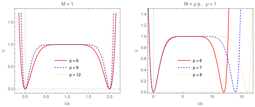
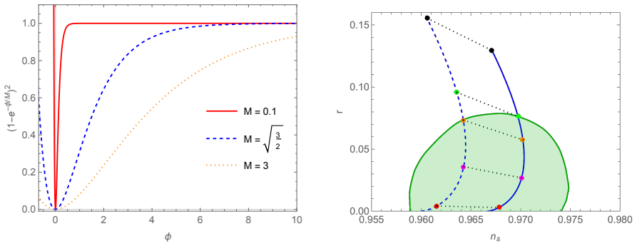
The central claim is that classes of inflationary SUGRA models need not differ by Kähler geometry or by superpotential; they can differ only by a field redefinition applied to the Kähler potential. For $K_-=-\frac12(f(T)-f(\bar T))^2+S\bar S$ and $W=\Lambda ST$, the F-term potential in canonically normalized variables $U=U_R+iU_I$ reduces, on the inflationary valley $U_I=0$, to $$V=\$Lambda^{2}$\left|$f^{{-1}}$\!\left(\frac{U_R}{\sqrt2}\right)\right|^2.$$ Thus the inverted function $f^{-1}$ is the inflaton potential shape. The paper's examples choose $f(T)=T^p$, $f(T)=\frac{M}{\sqrt2}(1-(1-T)^{1/p})$, $f(T)=-\frac{M}{\sqrt2}\log(1-T)$, $f(T)=\frac{M}{\sqrt2}e^T$, $f(T)=1/(\sqrt2 T)$, $f(T)=(aT+b)/(cT+d)$, and $f(T)=-\frac{1}{\sqrt2 M}\log^p T$, producing monomial, locally flat/hilltop, Starobinsky-like, log-squared, plateau, and bell-curve potentials. The paper states that this bypasses the earlier restriction that the function multiplying the stabilizer $S$ in $W$ be holomorphic, because at the level of the original $T$ field the superpotential stays the simple renormalizable $W=\Lambda ST$.
Load-bearing premise
The load-bearing premise is that redefining only the Kähler potential produces genuinely new SUGRA models, not just a change of variables that reproduces the previously known class of potentials.
Editorial extensions
If this is right
- The same flat Kähler geometry and the same superpotential $W=\Lambda ST$ can generate monomial, locally flat/hilltop, Starobinsky-like, log-squared, plateau, and bell-curve inflationary potentials, so the model type is no longer tied to the geometry or to a specially chosen superpotential.
- Predicted tensor-to-scalar ratios span $r\in[10^{-6},0.06]$ with $n_s$ within current bounds, so the family is differentiable with future CMB polarization measurements.
- The bell-curve model terminates inflation in a kination phase and reheats gravitationally at $T_R\sim\mathcal{O}(10^7\,\mathrm{GeV})$ without new couplings, giving a concrete link between inflationary observables and reheating.
- Because the manipulation is made on the Kähler potential for a general $G$, the same field-redefinition freedom can be applied to D-term inflation and to non-inflationary particle-phenomenology model building.
Reading between the lines
- Because $U=f(T)$ makes the canonical superpotential $W(U)=\Lambda S f^{-1}(U)$, that inverse function carries the whole potential shape; if $f^{-1}$ is not single-valued and holomorphic on the full field space, the model is a valid SUGRA theory only in a patch, or the procedure is a repackaging of the earlier holomorphic class.
- A natural next step would be to invert the dictionary: for any smooth single-field potential $V(\phi)$, solve $f^{-1}(\phi/\sqrt2)=\sqrt{V(\phi)}/\Lambda$ for $f$ and check whether the resulting Kähler potential is well-defined; this would map the method's true domain of applicability.
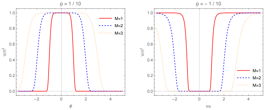
- The stark contrast between the $K_+$ and $K_-$ versions of the same $f$, for example Starobinsky-like versus natural inflation for $f\propto\log(1-T)$, shows that the sign choice is part of the model-building input, and a systematic scan over $f$ and sign could cover the reachable potentials.
Signed reviews
Editorial analysis
A structured set of objections, weighed in public.
Referee Report
Summary. The paper proposes a method to construct SUGRA inflationary models by applying a field redefinition f only to the Kähler potential, keeping the superpotential W = Λ S T fixed. After normalizing the field via U = f(T), the inflationary potential along the flat direction is claimed to be V = Λ^2 |f^{-1}(u_R/√2)|^2 (Eq. 12). The authors present several examples—monomial, locally flat/hilltop, Starobinsky-like, log-squared, plateau, modular, and bell-curve potentials—and compute their (n_s, r) predictions. The central claim is that this construction bypasses the holomorphicity restriction of earlier general-inflaton-potential constructions, specifically the Kallosh–Linde–Rube (KLR) class.
Significance. The explicit calculations are internally consistent and the models are valid SUGRA models with flat Kähler geometry. The paper provides a compact parametrization of several known inflationary potentials and adds a gravitational reheating mechanism for the bell-curve model. However, the claimed novelty does not hold: after canonicalization the superpotential remains holomorphic, and the resulting class is exactly the KLR class with holomorphic F. The paper's distinct contribution is therefore a set of worked examples and a coordinate reparametrization, not a new class of models or a bypass of holomorphicity.
major comments (3)
- [Section II, Eqs. (9)-(12)] The canonicalization U = f(T) requires f to be holomorphic for U to be a chiral superfield. In the U frame the superpotential is W = Λ S f^{-1}(U), which is holomorphic on suitable branches. Equation (12) is therefore exactly the KLR potential V = |F(u_R/√2)|^2 with F = Λ f^{-1}(U). The construction does not produce non-holomorphic superpotentials; it is a change of coordinates within the KLR class. The statements in the Introduction and Conclusions that the method 'bypasses the limit of holomorphicity' are not supported.
- [Sections III.A and III.D] The claims that the monomial and log-squared potentials 'could not be obtained using the standard K from [15]' are incorrect. KLR with holomorphic F(T) = T^{1/p} gives V ∝ φ^{2/p}, and with F(T) = log(T) gives V = log^2(u_R/√2). Thus these examples are already contained in [15], contradicting the paper's assertions, e.g., the statement in Section III.D that 'W ∝ log(T) is non-holomorphic.'
- [Conclusions, last paragraph] The closing claim that 'the idea of the field redefinition bypasses the limit of holomorphicity used for generating general potentials' is contradicted by the paper's own equations: the superpotential in the canonically normalized frame remains holomorphic. This is a load-bearing error because the paper's stated novelty rests on this point. The construction is a reparametrization of the KLR class, not a generalization beyond it.
minor comments (4)
- [Section II, Eq. (13)] Equation (13) is missing an equals sign; it should read ¨φ + 3H˙φ + V_φ = 0, and the subscript notation for the derivative should be made consistent.
- [Abstract and Conclusions] The statement that the models 'predict r ∈ [10^{-6}, 0.06]' is a range obtained by scanning free parameters M, p, n, and c/a; it is not a prediction of a single model. Consider rewording to 'models can cover r ∈ ...' to avoid overstating the result.
- [Section III.E] The generalization stated as 'f(T) = 1/(√2 T^{-n})' appears to be a typo; it should presumably be 'f(T) = T^{-n}/√2' to match the n = 1 case presented earlier.
- [Throughout] For non-integer powers p and for the modular transformation, the inverse function f^{-1} is multi-valued or has branch choices. The paper does not specify the chosen branches, so the superpotential is only locally defined; please add a clarifying statement.
Circularity Check
The central construction reduces to the known KLR class W=SF(T) by the field redefinition U=f(T), and the quoted r range is a parameter-scan envelope.
-
renaming known result
[Section II, Eqs. (9)-(12); Conclusions, final paragraph]
"To obtain a canonical Kähler metric let us introduce the following variable U = f(T) ⇒ T = f^{-1}(U) ... V = V− = Λ²|f^{-1}(u_R/√2)|². (12) ... The idea of the field redefinition bypasses the limit of holomorphicity used for generating general potentials by having an arbitrary holomorphic function f(T) in W."
For holomorphic f, U is a chiral superfield, so after canonicalization the theory has K = −½(U−Ū)²+|S|² and W = ΛS f^{-1}(U). This is exactly the Kallosh-Linde-Rube form W = S F(U) with F(U) = Λ f^{-1}(U), whose potential is V = |F(φ/√2)|². Thus Eq. (12) is the KLR potential by construction: the log-squared model is F = Λ log(√2 U/M), the monomial model is F = Λ U^{1/p}, and so on. No non-holomorphic superpotential is ever generated, so the claimed bypass of holomorphicity is not realized; the construction re-expresses the known KLR class in new coordinates and presents that renaming as a new class of theories.
-
fitted input called prediction
[Abstract; Section III G, Eqs. (52)-(53) and Fig. 11]
"The models are in accord with current observations and predict r∈[10^{-6},0.06] spanning several decades that can be easily obtained. ... the results of the (51) model may cover the whole 2σ regime of the Planck/BICEP data."
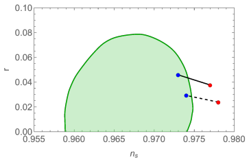
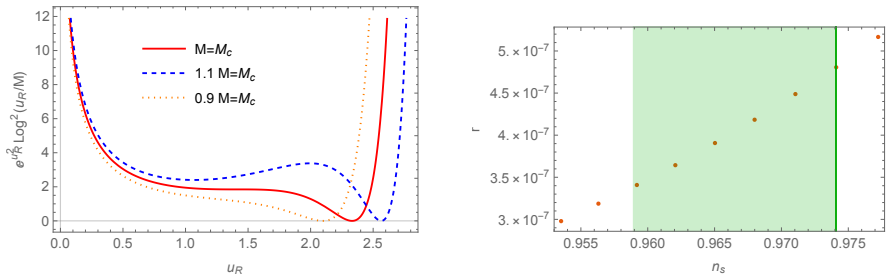
The parameters M and p (and in earlier models p, n, c/a) are free inputs that are varied in the figures. The quoted r range is the envelope of r values obtained by scanning these inputs over ranges chosen so that (n_s, r) stays inside Planck's 2σ region; Fig. 11, for instance, uses M ∈ {1,...,100} and p ∈ (−0.44, 0.16), etc. Hence 'predict r∈[10^{-6},0.06]' is a description of the scan range, not an independent model prediction. Similarly, saying that the bell-curve model can 'cover' the entire allowed (n_s,r) region is the definition of a free-parameter scan, not a parameter-free output of the construction.
full rationale
The derivation chain of the scalar potential is internally consistent, and the paper is not reliant on self-citation: the KLR class [15] is an external benchmark, while the authors' own citations [10,11,13,24,25,36,40] are not load-bearing for the main construction. However, the central novelty claim fails by the paper's own equations. Introducing U=f(T) in Eq. (9) and substituting into W=ΛST gives W=ΛS f^{-1}(U), which is precisely the KLR superpotential with F(U)=Λ f^{-1}(U). Equation (12), V=Λ²|f^{-1}(u_R/√2)|², is therefore the KLR potential V=|F(φ/√2)|² under a coordinate rename. In addition, the abstract's range r∈[10^{-6},0.06] is obtained by scanning free model parameters M, p, n, and c/a until the observables land inside the Planck 2σ region, so it has the status of a scan envelope rather than a prediction. These two issues make the paper substantially circular in its presentation of novelty, though the individual SUGRA models are valid and the computations are not definitionally identical to their inputs in a trivial tautological sense. Score 6 reflects one central reduction to a known result plus a scan-based 'prediction' presented as a model output.
Assumptions & free parameters
free parameters (6)
- Λ (overall mass scale) =
unfixed
- M (mass scale inside f) =
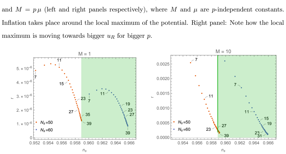
model-dependent: 1 to 100; Starobinsky M < 11 or 17.5
- p (exponent in f) =
hilltop p ∈ (7, 39); bell-curve p ∈ (−1.7, 0.16)
- n (plateau exponent) =
1, 2, 4
- c/a (modular transformation ratio) =
1 to 20 or 1/3 to 10
- N⋆ (number of e-folds) =
50 or 60
assumptions (5)
- standard math F-term scalar potential V = e^G(K^{iĵ}D_i W D_ĵ W̅ − 3|W|²) and integration of the stabilizer S at S = 0 gives V = e^K|W_S|².
- domain assumption Kähler potential ansatz K± = ±½(f(T) ± f(T̄))² + SS̄ with W = ΛST, and the S field can be integrated out supersymmetrically.
- ad hoc to paper f(T) is holomorphic and f⁻¹ defines a valid holomorphic superpotential on the field space, including branch choices for noninteger powers.
- ad hoc to paper The transformation T → f(T) applied only to K produces a new theory not equivalent to the full field redefinition or to [15].
- domain assumption Slow-roll approximation with N⋆ = 50 or 60 e-folds.
Cite this review
Pith. "Pith review of Inflation in supergravity from field redefinitions." pith.science (2026). https://pith.science/paper/CKKG5C6N
@misc{pith2026190807052,
  author       = {Pith},
  title        = {Pith review of: Inflation in supergravity from field redefinitions},
  year         = {2026},
  howpublished = {\url{https://pith.science/paper/CKKG5C6N}},
  note         = {Machine review of arXiv:1908.07052}
}
abstract
Supergravity (SUGRA) theories are specified by a few functions, most notably the real K\"ahler function denoted by $G(T_i, \bar {T}_i) = K + \log |W|^2$, where K is a real K\"ahler potential, and W is a holomorphic superpotential. A field redefinition $T_i \rightarrow f_1(T_i)$ does not change neither the theory, nor the K\"ahler geometry. Similarly, the K\"ahler transformation, $K \rightarrow K + f_2 + \bar f_2, W \rightarrow e^{-f_2} W$ where $f_2$ is holomorphic also leaves G and hence the theory and the geometry invariant. However, if we perform a field redefinition only in $K(T_i,\bar{T}_i) \rightarrow K(f(T_i),f(\bar{T}_i))$, while keeping the same superpotential $W(T_i)$, we get a different theory, as G is not invariant under such a transformation while maintaining the same K\"ahler geometry. This freedom of choosing $f(T_i)$ allows constructing an infinite number of new theories given a fixed K\"ahler geometry and a predetermined superpotential W. Our construction generalizes previous ones that were limited by the holomorphic property of $W$. In particular it allows for novel inflationary SUGRA models and particle phenomenology model building, where the different models correspond to different choices of field redefinitions. We demonstrate this possibility by constructing several prototypes of inflationary models (hilltop, Starobinsky-like, plateau, log-squared and bell-curve) all in flat K\"ahler geometry and an originally renormalizable superpotential $W$. The models are in accord with current observations and predict $r\in[10^{-6},0.06]$ spanning several decades that can be easily obtained. In the bell-curve model, there also exists a built-in gravitational reheating mechanism with $T_R\sim \mathcal{O}( 10^7 GeV)$.
Figures
Figures from the paper (8 more)



Reference graph
Works this paper leans on
-
[15]
Volume modulus inflation and a low scale of SUSY breaking
Badziak, M.; Olechowski, M. Volume modulus inflation and a low scale of SUSY breaking. 22 JCAP 2008, 807, 21
work page 2008
-
[1]
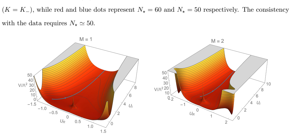
The scalar potential V+ as a function of uR and uI is presented in the Figure 5
The K =K+ Scenario This model has this interesting feature, where both V+ and V− may generate successful inflation. The scalar potential V+ as a function of uR and uI is presented in the Figure 5. In the case of K = K+ the evolution of fields may look more complicated. First, the field reaches the uR = 0 valley, for which the inflationary potential may be app...
-
[2]
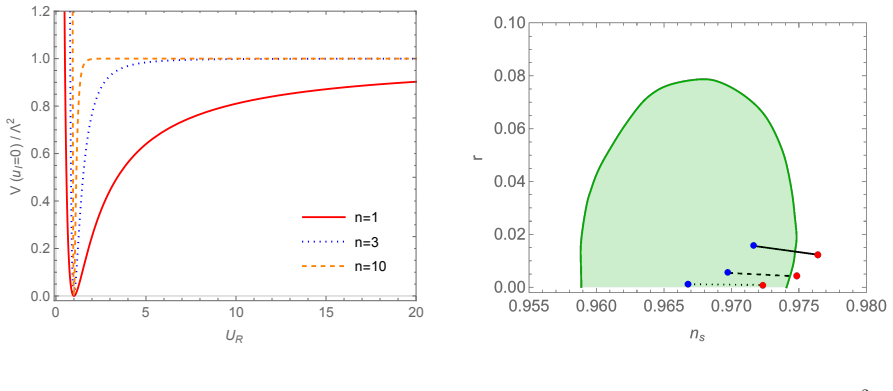
Solid, dashed and dotted lines correspond to n = 1, n = 2 and n = 4 respectively. One can simplify this potential using ad−bc = 1 and a simple field transformation uR→uR + √ 2a/c, which gives V = Λ2d2 c2 ( 1 + √ 2 cd 1 uR )2 . (43) The (43) model is simply a generalization of the (38). On the other hand, for K =K+ one finds V (uR = 0) = Λ2 2b2 +d2u2 I 2a2 +...
-
[3]
Within the slow-roll approximation one finds r ≃ 16 2N⋆(1− 2p) (√ 2M|p| ) 1 1−p + 1 − 2(1−p) 1−2p (52) ns ≃ 1− 2 2N⋆(1− 2p) (√ 2M|p| ) 1 1−p + 1 − 2(1−p) 1−2p − 4(1−p) (√ 2M|p| ) 1 1−p + 2N⋆(1− 2p) . (53) Please note that in the N⋆≪ 1 2(1− 2p) (√ 2M|p| ) 1 1−p (54) regime equation (52) takes the form of ϵ≃ ϵ0 Nn, (55) 18 whereM = (2p−1)√ϵ0(...
-
[4]
A New Type of Isotropic Cosmological Models Without Singularity
Starobinsky, A.A. A New Type of Isotropic Cosmological Models Without Singularity. Phys. Lett. 1980, 91, 99
work page 1980
-
[5]
Particle physics models of inflation and the cosmological density per- turbation
Lyth, D.H.; Riotto, A. Particle physics models of inflation and the cosmological density per- turbation. Phys. Rep. 1999, 314, 1
work page 1999
-
[6]
First Order Phase Transition of a Vacuum and Expansion of the Universe
Sato, K. First Order Phase Transition of a Vacuum and Expansion of the Universe. Mon. Not. Roy. Astron. Soc. 1981, 195, 467
work page 1981
-
[7]
The Inflationary Universe: A Possible Solution to the Horizon and Flatness Prob- lems
Guth, A.H. The Inflationary Universe: A Possible Solution to the Horizon and Flatness Prob- lems. Phys. Rev. D 1981, 23, 347
work page 1981
Show all 43 references
-
[8]
Planck 2018 results
Akrami, Y.; Arroja, F.; Ashdown, M.; Aumont, J.; Baccigalupi, C.; Ballardini, M.; Banday, A.J.; Barreiro, R.B.; Bartolo, N.; Basak, S.; et al. Planck 2018 results. X. Constraints on inflation. arXiv 2018, arXiv:1807.06211
2018 arXiv
-
[9]
Superconformal Inflationary α-Attractors
Kallosh, R.; Linde, A.; Roest, D. Superconformal Inflationary α-Attractors. JHEP 2013, 1311, 198, doi:10.1007/JHEP11(2013)198
2013 doi
-
[10]
Endlessly flat scalar potentials and α-attractors
Artymowski, M.; Rubio, J. Endlessly flat scalar potentials and α-attractors. Phys. Lett. B 2016, 761, 111, doi:10.1016/j.physletb.2016.08.024
2016 doi
-
[11]
Initial conditions for inflation
Dimopoulos, K.; Artymowski, M. Initial conditions for inflation. Astropart. Phys. 2017, 94, 11, doi:10.1016/j.astropartphys.2017.06.006
2017 doi
-
[12]
Natural chaotic inflation in supergravity
Kawasaki, M.; Yamaguchi, M.; Yanagida, T. Natural chaotic inflation in supergravity. Phys. Rev. Lett. 2000, 85, 3572
2000
-
[13]
Supergravity Higgs Inflation and Shift Symmetry in Electroweak Theory
Ben-Dayan, I.; Einhorn, M.B. Supergravity Higgs Inflation and Shift Symmetry in Electroweak Theory. JCAP 2010, 1012, 2
2010
-
[14]
Higgs Chaotic Inflation in Standard Model and NMSSM
Nakayama, K.; Takahashi, F. Higgs Chaotic Inflation in Standard Model and NMSSM. JCAP 2011, 1102, 10
2011
-
[16]
Models of Modular Inflation and Their Phenomeno- logical Consequences
Ben-Dayan, I.; Brustein, R.; de Alwis, S.P. Models of Modular Inflation and Their Phenomeno- logical Consequences. JCAP 2008, 807, 11
2008
-
[17]
Constraints on modular inflation in supergravity and string theory
Covi, L.; Gomez-Reino, M.; Gross, C.; Louis, J.; Palma, G.A.; Scrucca, C.A. Constraints on modular inflation in supergravity and string theory. JHEP 2008, 808, 55
2008
-
[18]
General inflaton potentials in supergravity
Kallosh, R.; Linde, A.; Rube, T. General inflaton potentials in supergravity. Phys. Rev. D 2011, 83, 43507
2011
-
[19]
Emergent Weyl spinors in multi-fermion systems
Volovik, G.; Zubkov, M. Emergent Weyl spinors in multi-fermion systems. Nucl. Phys. B 2014, 881, 514–538
2014
-
[20]
Chiral anomaly, dimensional reduction, and magne- toresistivity of Weyl and Dirac semimetals
Gorbar, E.; Miransky, V.; Shovkovy, I. Chiral anomaly, dimensional reduction, and magne- toresistivity of Weyl and Dirac semimetals. Phys. Rev. B 2014, 89, 85126
2014
-
[21]
Torsion, Parity-odd Response and Anomalies in Topological States
Parrikar, O.; Hughes, T.L.; Leigh, R.G. Torsion, Parity-odd Response and Anomalies in Topological States. Phys. Rev. D 2014, 90, 105004
2014
-
[22]
Stability of Fermi surfaces and K-theory
Horava, P. Stability of Fermi surfaces and K-theory. Phys. Rev. Lett. 2005, 95, 16405
2005
-
[23]
The Universe in a helium droplet
Volovik, G. The Universe in a helium droplet. Int. Ser. Monogr. Phys. 2006, 117, 1–526
2006
-
[24]
Unity of Cosmological Inflation Attractors
Galante, M.; Kallosh, R.; Linde, A.; Roest, D. Unity of Cosmological Inflation Attractors. Phys. Rev. Lett. 2015, 114, 141302
2015
-
[25]
Probing the BSM physics with CMB precision cosmology: An application to supersymmetry
Dalianis, I.; Watanabe, Y. Probing the BSM physics with CMB precision cosmology: An application to supersymmetry. JHEP 2018, 2, 118
2018
-
[26]
Hilltop inflation
Boubekeur, L.; Lyth, D.H. Hilltop inflation. JCAP 2005, 507, 10
2005
-
[27]
Accidental inflation from K¨ ahler uplifting
Ben-Dayan, I.; Jing, S.; Westphal, A.; Wieck, C. Accidental inflation from K¨ ahler uplifting. JCAP 2014, 1403, 54
2014
-
[28]
Cosmic Microwave Background Observables of Small Field Models of Inflation
Ben-Dayan, I.; Brustein, R. Cosmic Microwave Background Observables of Small Field Models of Inflation. JCAP 2010, 1009, 7
2010
-
[29]
Realising Mutated Hilltop Inflation in Supergravity
Pinhero, T.; Pal, S. Realising Mutated Hilltop Inflation in Supergravity. Phys. Lett. B 2019, 796, 220
2019
-
[30]
Saddle point inflation in string-inspired theory
Hamada, Y.; Kawai, H.; Kawana, K. Saddle point inflation in string-inspired theory. PTEP 2015, 2015, 91B01
2015
-
[31]
Large field inflation and double α-attractors
Kallosh, R.; Linde, A.; Roest, D. Large field inflation and double α-attractors. JHEP 2014, 1408, 52
2014
-
[32]
Superconformal generalizations of the Starobinsky model
Kallosh, R.; Linde, A. Superconformal generalizations of the Starobinsky model. JCAP 2013, 23 1306, 28
2013
-
[33]
Planck constraints on single-field inflation
Tsujikawa, S.; Ohashi, J.; Kuroyanagi, S.; Felice, A.D. Planck constraints on single-field inflation. Phys. Rev. D 2013, 88, 23529
2013
-
[34]
Natural α-Attractors fromN = 1 Supergravity via flat K¨ ahler Manifolds.arXiv 2018, arXiv:1812.05406
Pinhero, T. Natural α-Attractors fromN = 1 Supergravity via flat K¨ ahler Manifolds.arXiv 2018, arXiv:1812.05406
2018 arXiv
-
[35]
Natural inflation: Particle physics models, power law spectra for large scale structure, and constraints from COBE.Phys
Adams, F.C.; Bond, J.R.; Freese, K.; Frieman, J.A.; Olinto, A.V. Natural inflation: Particle physics models, power law spectra for large scale structure, and constraints from COBE.Phys. Rev. D 1993, 47, 426
1993
-
[36]
Inflation without Selfreproduction
Mukhanov, V. Inflation without Selfreproduction. Fortsch. Phys. 2015, 63, 36
2015
-
[37]
Instant preheating
Felder, G.N.; Kofman, L.; Linde, A.D. Instant preheating. Phys. Rev. D 1999, 59, 123523
1999
-
[38]
Gravitational Particle Creation and Inflation
Ford, L.H. Gravitational Particle Creation and Inflation. Phys. Rev. D 1987, 35, 2955
1987
-
[39]
Gravitational wave signals and cos- mological consequences of gravitational reheating
Artymowski, M.; Czerwinska, O.; Lalak, Z.; Lewicki, M. Gravitational wave signals and cos- mological consequences of gravitational reheating. JCAP 2018, 1804, 46
2018
-
[40]
Role of trans-Planckian modes in cosmology
Berera, A.; Brahma, S.; Calder ˘A ln, J.R. Role of trans-Planckian modes in cosmology. arXiv 2003, arXiv:2003.07184
2003 arXiv
-
[41]
Trans-Planckian censorship conjecture from the swampland distance conjecture
Brahma, S. Trans-Planckian censorship conjecture from the swampland distance conjecture. Phys. Rev. D 2020, 101, 46013
2020
-
[42]
A refined trans-Planckian censorship conjecture
Cai, R.; Wang, S. A refined trans-Planckian censorship conjecture. arXiv 2019, arXiv:1912.00607
2019 arXiv
-
[43]
Draining the Swampland
Ben-Dayan, I. Draining the Swampland. Phys. Rev. D 2019, 99, 101301. 24
2019
Reviewed August 14, 2026 · model on record in the stance chip above.
Discussion (0). Continue with ORCID to comment.