REVIEW 4 major objections 6 minor 49 references
A Quantum Ring in a Nanosphere
T0 review · 4 major / 6 minor · reviewed 2026-08-14 · deepseek-v4-flash
Pith's one-line read This paper claims the Schrödinger equation for a quantum ring on a sphere with a magnetic field and Aharonov-Bohm flux is exactly solvable, yielding closed-form energies, magnetization, and persistent current.
desk verdict The spherical Tan–Inkson ring paper is a plausible extension, but as written the central spectrum contradicts the paper's own quantization condition and the advertised uniform magnetic field is not uniform. read the letter →
The pith
A machine-rendered reading of the paper's core claim, the machinery that carries it, and where it could break.
The reading
What carries the argument
The central object is the curved Tan-Inkson confinement potential (9), a harmonic well whose minimum sits at radius $\rho_0$. The calculation is carried by the coordinate substitution $x=1/[1+(\rho/2a)^2]$, the stereographic coordinate on the sphere, which turns the radial equation into a hypergeometric equation of the form (24). The key identifications $\alpha=\mu a^2\omega_m/\hbar$ and $\gamma=M/2$ let the polynomial-solution condition (35) become the closed-form spectrum (36). The derived frequency $\omega_m$ (21) and angular number $M$ (20) pack the combined effects of curvature, magnetic field, and confinement into one exactly solvable equation.
What would settle it
Compute the physical field strength from the vector potential (5) using the metric (4): if the magnitude varies with $\rho$ and diverges as $\rho\to 0$, the Hamiltonian solved is not a ring in a uniform magnetic field, so Eqs. (36), (46), and (53) do not describe the stated physical system. A measurement of energy levels on a curved ring under a genuinely uniform field would then disagree with Eq. (36).
Extended reading notes
Core claim
The paper's central claim is that the Hamiltonian (14), describing a particle on a sphere in stereographic coordinates under the vector potentials (5) and (6) together with the curved Tan-Inkson potential (9), has an exactly solvable Schrödinger equation. The energy levels are $$E = \frac{\$hbar^{2}$}{2\mu $a^{2}$}\left[\left(n+\frac12\right)^2 + \left(n+\frac12\right) M + \frac12\left(m+\frac{\Phi_{AB}}{\Phi_0}\right)^2\right] + \hbar\omega_m\left(n+\frac12+\frac{M}{2}\right) + \hbar\omega_c\left(m+\frac{\Phi_{AB}}{\Phi_0}\right) - \frac{\mu\$omega_0^{2}$\$rho_0^{2}$}{4},$$ with $M$ and $\omega_m$ defined in Eqs. (20) and (21). The corresponding wavefunctions are hypergeometric polynomials of the form (33). From this spectrum the paper derives the magnetization at $T=0$ (Eq. (46)) and the persistent current (Eq. (53)), and it checks the result against the flat Tan-Inkson ring in the limit $a\to\infty$ and against Landau levels on a sphere when confinement and flux are absent.
Load-bearing premise
The paper's results all rest on the vector potential in Eq. (5) being a uniform magnetic field on the sphere; if that field is not actually uniform, the solved spectrum does not describe the advertised quantum ring.
Editorial extensions
If this is right
- The spectrum (36) is not simply the flat-ring spectrum rescaled: curvature enters through the prefactor $1/a^2$, through $M$, and through $\omega_m$, so the spacing between levels changes with the sphere radius.
- The persistent current (53) contains a curvature-dependent term proportional to $\omega_c/\omega_m$ that breaks the direct proportionality between magnetic moment and current, a deviation that is absent in the purely flat model.
- In the limit $a\to\infty$ the formulas reproduce the flat Tan-Inkson ring, and in the limit $\lambda_1=\lambda_2=0$, $\Phi_{AB}=0$ they reproduce Landau levels on a sphere, giving two independent checks of the exact solution.
- Because the spectrum is discrete, the model describes a bound ring rather than a conduction band; the paper notes this stands in contrast to the hyperbolic-space version of the same construction, where continuous eigenvalues also occur.
Reading between the lines
- If the exact solution is taken as a method, the same $x$-substitution only yields a solvable hypergeometric equation for potentials of Tan-Inkson type; for a generic radial potential on the sphere the problem is not exactly solvable, so the special form of the potential, not the sphere geometry alone, is what carries the solubility.
- A direct test would be to compute the Aharonov-Bohm periodicity of the magnetization and current from Eqs. (46) and (53): the flux enters both additively and through $M$ and $\omega_m$, so the response is expected to deviate from pure $\Phi_0$-periodicity as curvature increases—an effect the paper does not explicitly analyze.
- Because the spectrum is closed-form, a finite-temperature or many-particle version of the magnetization can be obtained by summing Eq. (43) over the Fermi distribution without further approximation, which would connect the curvature dependence to experimentally measured thermodynamic quantities.
Signed reviews
Editorial analysis
A structured set of objections, weighed in public.
Referee Report
Summary. The paper studies a charged particle confined to a spherical surface (stereographically projected metric) with a Tan–Inkson-type confining potential, an Aharonov–Bohm flux, and a magnetic field, claiming an exact solution of the Schrödinger equation. The energy eigenvalues (36) and eigenfunctions (33) are presented, and from them the zero-temperature magnetization (46) and persistent current (53) are derived, with flat-space limits claimed. The paper's main claims are: (i) exact solvability of Hamiltonian (14); (ii) reduction to the flat Tan–Inkson spectrum as a→∞; (iii) new curvature-dependent terms in magnetization and persistent current.
Significance. If correct, the result would extend the exactly solvable Tan–Inkson quantum ring model to a positively curved geometry and would give concrete predictions for magnetization and persistent currents, usable for comparison with forthcoming experiments on curved nanostructures. The manuscript's strengths are its ambition to provide closed-form results extending a well-known solvable model, and its effort to present the flat-space and zero-confinement limits. The claimed Landau-level limit (Dunne) and the Tan–Inkson flat limit are clearly stated falsifiable predictions. However, these strengths cannot be realized unless the derivation is internally consistent and the magnetic field is that announced in the model.
major comments (4)
- [IV, Eqs. (30)–(36)] The central energy formula (36) does not follow from the stated quantization condition. With α defined in (30), γ in (31), and β(1−β) in (32), the termination condition α+β+γ = −n fixes β = −n−α−γ. Substituting into (32), expanding α and γ with (20)–(21) and ω_0^2 from (18), yields E = (ℏ^2/(2μa^2))[(n+1/2)^2 + (n+1/2)M + q^2/2] + ℏω_m(n+1/2+M/2) + (ℏ/2)ω_c q − μω_0^2ρ_0^2/4, with q = m + Φ_AB/Φ_0. The published formula (36) has ℏω_c q instead of (ℏ/2)ω_c q. For ℏ=μ=a=1, ω_c=ω_0=1, q=1, ρ_0/(2a)=1, n=0, the termination condition gives E ≈ 3.351 while (36) gives ≈ 3.851. Since (36) is the basis for the magnetization (46) and persistent current (53), this coefficient error propagates through the two central physical results.
- [II, Eq. (5)] The vector potential (5) does not describe a uniform magnetic field on the sphere. The physical field F = dA in the metric (4) has field strength F_{ρφ} = B(1 − 3ρ^2/(4a^2))/(2ρ[1+(ρ/2a)^2]^3), which is position dependent and diverges as ρ→0. Thus the Hamiltonian actually solved (14) is not the uniform-field ring Hamiltonian announced in the abstract and introduction. If the intended gauge were dA = B dS with constant B on the surface, the gauge-dependent terms in (8) would have different factors of [1+(ρ/2a)^2], and the spectrum (36) and all derived thermodynamics would change.
- [IV, Eq. (35) and following line] The quantization condition (35) is stated as an inequality, α+β+γ ⩽ −n, used by solving condition (35) when equality holds, but the bound on n given after (36), 0 ⩽ n < μω_m a^2/ℏ − M/2 − 1/2, is asserted without proof. Since α itself depends on n-dependent parameters through ω_m in (30), the termination condition and the stated bound on n must be derived consistently; the manuscript does not show that the hypergeometric series terminates at the claimed integer n, nor that the polynomial normalization holds at that n. This is needed to confirm that (33) is a normalizable eigenfunction of (14) rather than a formal solution.
- [VI, Eqs. (49)–(50)] The derivative formulas (49)–(50) contain apparent typos that undermine the persistent-current derivation. Eq. (49) as written, ∂M/∂Φ_AB = (1/2)(1/M^2)(m+Φ_AB/Φ_0)(1/Φ_0) = (1/M)(m+Φ_AB/Φ_0)(1/Φ_0), is dimensionally inconsistent and oscillates between 1/M^2 and 1/M; the correct derivative of M in (20) is (1/2M)(m+Φ_AB/Φ_0)(1/Φ_0). Eq. (50) begins with an equality ∂ω_m/∂Φ_AB = 2(m+Φ_AB/Φ_0)(1/Φ_0) that is dimensionally wrong and is then re-expressed; the intermediate equality is not the derivative of (21). These errors make the route from (48) to (51)–(53) unreliable, independently of the issues in the spectrum.
minor comments (6)
- [Abstract and Section I] The abstract and the sentence introducing Section IV contain duplicated wording (the magnetization and persistent current are calculated appearing twice in consecutive sentences in the abstract), and the introduction should be copy-edited for typos such as persistent current is f calculated in the last paragraph of Section I.
- [Eq. (16)] Equation (16) is not self-contained: the transformation (15) is not used consistently to express the kinetic term, and the potential terms appear without explanation of the intermediate algebraic steps. Please provide the derivation from (14) to (19) in full, or at least state the simplification leading to (19).
- [Eqs. (30) and (34)] The notation is unclear at Eqs. (30)–(34): α is defined with the sign convention (30), while the square root in (34) should be labelled ±β with the chosen α; the paper would benefit from an explicit statement of how the sign in (34) is fixed and how (35) selects the physical branch.
- [Eq. (37)] The flat limit (37) is suspect as written: ω_fm = sqrt[(ω_c^2+ω_0)^2] appears to be missing squares and the factor 1/2 in the ω_c term. Please verify the flat limit formula against Tan and Inkson and state which version of the cyclotron frequency (SI versus Gaussian CGS) is used, as the discussion in reference [47] acknowledges ambiguity.
- [V, Eq. (43)] The first equality in the magnetization derivation (42) is followed by a result (43) with a factor m_0/μ; the ratio m_0/μ is not defined at this point and the sign conventions should be stated explicitly, since the persistent current (53) depends on the sign of the magnetization.
- [VI, Eq. (53)] The final persistent-current formula (53) is written compactly; please show how the factor [1+(ρ_m/2a)^2] arises from combining (51) with (54), and specify whether the result is in Gaussian CGS units (since c appears explicitly throughout).
Circularity Check
No circularity found: spectrum, magnetization, and persistent current are derived directly from the stated Hamiltonian without fitted inputs or load-bearing self-citations.
full rationale
The paper's central derivation is self-contained: the Hamiltonian (14) is combined with the ansatz (16), transformed to the variable x, and reduced to the hypergeometric equation (23)/(24). The quantization condition (35) then yields the energy eigenvalues (36). The magnetization (46) is obtained by taking the derivative of this energy spectrum with respect to the magnetic field, and the persistent current (53) follows from the Byers-Yang relation. No parameter is fitted to data, and no previously published result is used as an unverified premise: the hypergeometric solution is standard mathematical theory, and the Byers-Yang relation is cited from the original external literature. The cited limits (Tan-Inkson flat limit, Dunne Landau levels on a sphere) are stated as comparisons/checks, not as inputs to the derivation. The authors' self-citations in the introduction and conclusions are contextual and are not load-bearing for the central result. The skeptic's point that Eq. (36) may be algebraically inconsistent with the termination condition (35), or that the vector potential (5) may not describe a uniform field, concerns correctness of the derivation, not circularity: an erroneous step is not the same as a step that reduces to its own inputs. Therefore there is no significant circularity in the paper's claimed derivation chain.
Assumptions & free parameters
assumptions (4)
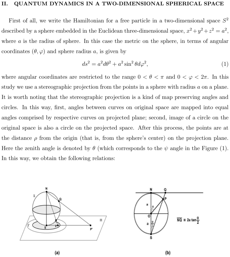
- standard math The metric after stereographic projection is ds^2 = (d(rho)^2 + rho^2 d(phi)^2)/(1 + (rho/2a)^2)^2 (Eq. 4); the sphere radius a is the only curvature scale.
- domain assumption The vector potential A1 in Eq. (5) is supposed to represent a uniform magnetic field on the sphere; the physical field is not computed in the paper, but the Hamiltonian is built from this gauge.
- ad hoc to paper The Tan-Inkson potential in spherical coordinates, Eq. (9), with the specific constant V0 in Eq. (10), is the exact model for the quantum ring; this potential is constructed so the radial equation maps to a hypergeometric equation.
- standard math The hypergeometric function solution terminates via the condition alpha + beta + gamma <= -n, and the square-integrable states are those with 0 <= n < mu omega_m a^2/hbar - M/2 - 1/2.
Cite this review
Pith. "Pith review of A Quantum Ring in a Nanosphere." pith.science (2026). https://pith.science/paper/CFOR6SJE
@misc{pith2026190809956,
  author       = {Pith},
  title        = {Pith review of: A Quantum Ring in a Nanosphere},
  year         = {2026},
  howpublished = {\url{https://pith.science/paper/CFOR6SJE}},
  note         = {Machine review of arXiv:1908.09956}
}
read the original abstract
In this paper we study the quantum dynamics of an electron/hole in a two-dimensional quantum ring within a spherical space. For this geometry, we consider a harmonic confining potential. Suggesting that the quantum ring is affected by the presence of an Aharonov-Bohm flux and an uniform magnetic field, we solve the Schr\"odinger equation for this problem and obtain exactly the eigenvalues of energy and corresponding eigenfunctions for this nanometric quantum system. Afterwards, we calculate the magnetization and persistent current are calculated, and discuss influence of curvature of space on these values.
Figures
Reference graph
Works this paper leans on
-
[1]
Aharonov and D
Y. Aharonov and D. Bohm, Phys. Rev. 115, 485 (1959)
1959
-
[2]
U. F. Keyser et al, Semicond. Sci. Technol. 17, L22 (2002)
work page 2002
-
[3]
Y. Meir, O. Entin-Wohlman, Y. Gefen, Phys. Rev. B 42, 8351 (1990)
work page 1990
-
[4]
W. C. Tan and J. C. Inkson, Phys. Rev. B 60, 5626 (1999)
work page 1999
- [5]
-
[6]
B. I. Halperin, Phys. Rev. B 25, 2185 (1982)
1982
- [7]
- [8]
Show all 49 references
-
[9]
W. C. Tan and J. C. Inkson, Semicond. Sci. and Technol. 11, 1635 (1996)
1996
-
[10]
V. A. Margulis, A. V. Shorokhov, and M. P. Trushin, Physica E 10, 518 (2001)
2001
-
[11]
E. N. Bogachek and U. Landman, Phys. Rev. B 52, 14067 (1995)
1995
-
[12]
M. V. Berry, J. P. Keating, J. Phys. A 27, 6167 (1994)
1994
-
[13]
V. Y. Prinz, V. A. Seleznev, A. K. Gutakovsky, A. V. Chehovskiy, V. V. Preobrazhenskii, M. A. Putyato, T. A. Gavrilova, Physica E 6, 828 (2000)
2000
-
[14]
G. V. Dunne, Ann. Phys. (N.Y.) 215, 233 (1992)
1992
-
[15]
Comtet, P
A. Comtet, P. J. Houston, J. Math. Phys. 26, 185 (1985)
1985
-
[16]
A. Comtet. Ann. Phys. (N.Y.) 173, 185 (1987)
1987
-
[17]
Greiter, Phys
M. Greiter, Phys. Rev. B 83, 115129 (2011)
2011
-
[18]
D. V. Bulaev, V. A. Geyler and V. A. Margulis, Phys. Rev. B 337, 180 (2003)
2003
-
[19]
T. Mine, Y. Nomura, J. Funct. Anal. 263 1701 (2012)
2012
- [20]
- [21]
-
[22]
V. P. Nair, J. Phys. A39, 12735 (2006), hep-th/0606161
2006 arXiv
-
[23]
Hasebe, Phys
K. Hasebe, Phys. Rev. D 78, 125024 (2008)
2008
- [24]
-
[25]
V. P. Nair, S. Randjbar-Daemi, Nucl. Phys. B679, 447 (2004)
2004
- [26]
- [27]
-
[28]
V. Y. Prinz, D. Gr¨ utzmacher, A. Beyer, C. David, B. Ketterer, and E. Deccard, in Proccedings of 9th International Symposium Nanostructures: Physics and Technology (St. Petersburg, Russia, 2001), p. 13
2001
-
[29]
C. L. de Souza Batista, D. Li, Phys. Rev. B 55, 1582 (1997)
1997
-
[30]
A. L. Carey, K. C. Hannabuss, V. Mathai, P. McCann, Commun. Math. Phys. 190, 629 (1998)
1998
-
[31]
M. L. Leadbeater, C. L. Forden, T. M. Burke, J. H. Burroughes, M. P. Grimshaw, D. A. Ritchie, L. L. Wang, M. Pepper, J. Phys.: Cond. Mat. 7, L307 (1995)
1995
-
[32]
M. V. Entin, L. I. Magarill, Phys. Rev. B 64, 085330 (2001)
2001
-
[33]
D. V. Bulaev and V.A. Margulis, Eur. Phys. J. B. 36, 183 (2003)
2003
-
[34]
Geyler, P
V. Geyler, P. Stovicek, M. Tusek, Operator Theory: Advances and Applications, 188, 135 (2008)
2008
-
[35]
Geyler, P
V. Geyler, P. Stovicek, J. Phys. A: Math. and Gen. 36, 1375 (2006)
2006
-
[36]
D. V. Bulaev, V. A. Geyler and V.A. Margulis, Phys. Rev. B 62, 11517 (2000)
2000
-
[37]
Furtado, A
C. Furtado, A. Rosas, S. Azevedo, Europhys. Lett. 79, 57001 (2007)
2007
-
[38]
A. L. Silva Netto, C. Chesman and C. Furtado, Phys. Lett. A 372, 3894 (2008)
2008
-
[39]
Dantas, A
L. Dantas, A. L. Silva Netto and C. Furtado, Phys. Lett. A 379, 11 (2014)
2014
-
[41]
L. D. Landau, E, M. Lifshitz, Quantu Mechanics, Pergamon Press, Oxford, 1980
1980
-
[42]
J. J. Sakurai, Modern Quantum Mechanics, Addison-Wesley Publishing Company, 1994
1994
-
[43]
Furtado, C
C. Furtado, C. A. de Lima Ribeiro, S. Azevedo, Phys. Lett. A 296, 171 (2002)
2002
-
[44]
G. V. Dunne, Hilbert Space for Charged Particles in Perpendicular Magnetic Fields , Ann. Phys. 215, 233 (1992)
1992
-
[45]
Rubinowicz, Sommerfeld’s Polynomial Method Simplified , Proceedings of the Physical So- ciety, Section A 63 (7), 766 (1950)
A. Rubinowicz, Sommerfeld’s Polynomial Method Simplified , Proceedings of the Physical So- ciety, Section A 63 (7), 766 (1950). 15
1950
-
[46]
L. D. Landau, E. M. Lifshitz, Statistical Physics, Pergamon Press, Oxford, 1980
1980
-
[47]
units and the factor ℏe µ in [9]? would be similar to the relation (43) in our contribution except for a 1 c factor that comes from Gaussian CGS units choice
F romreference [4], one sees that according to relations 4, ωc is defined for S.I. units and the factor ℏe µ in [9]? would be similar to the relation (43) in our contribution except for a 1 c factor that comes from Gaussian CGS units choice. In the rest of the paper , if we con...
-
[48]
Byers, C
N. Byers, C. N. Yang, Phys. Rev. Lett. 7, 46 (1961)
1961
-
[49]
J. D. Jackson, Classical Electrodynamics (John Wiley & Sons, Inc. New York, 1999), 3rd edition, p. 183
1999
-
[50]
J. Liu, W. X. Gao, K. Ismail, K. Y. Lee, J. M. Hong, and S. Washburn, Phys. Rev. B 48, 148 (1993). 16
1993
Reviewed August 14, 2026 · model on record in the stance chip above.
Discussion (0). Continue with ORCID to comment.