REVIEW 3 major objections 4 minor 50 references
2D numerical simulation of lunar response to gravitational waves using finite element method
T0 review · 3 major / 4 minor · reviewed 2026-08-11 · deepseek-v4-flash
Pith's one-line read The paper establishes that a two-dimensional finite-element simulation of the Moon reproduces semi-analytical gravitational-wave response functions, making numerical lunar GW seismology with realistic structure a feasible next step.
desk verdict First SEM simulation of lunar GW response, but validation rests on an underived frequency shift. read the letter →
The pith
A machine-rendered reading of the paper's core claim, the machinery that carries it, and where it could break.
The reading
What carries the argument
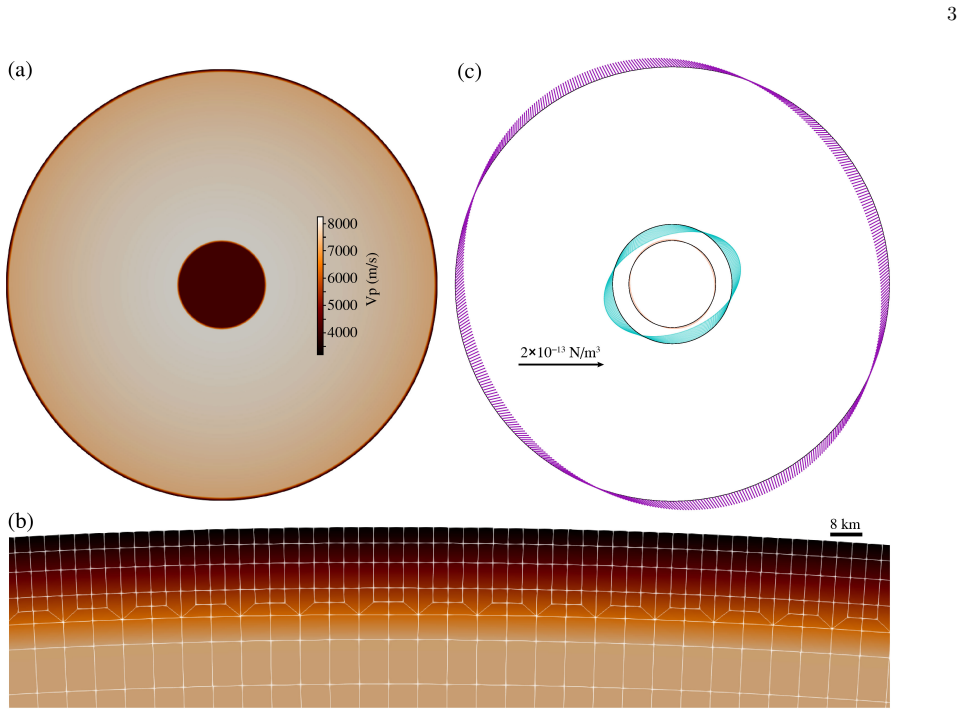
The simulation is carried out with a two-dimensional spectral element method, a high-order finite-element technique, on a global lunar model built from 140,576 fourth-order elements with a mesh that grows coarser with seismic wave speed; the grid resolves frequencies up to about 0.2 Hz. The gravitational wave enters through the force density $\vec{f}=\nabla\mu\cdot h$, where $\mu$ is the shear modulus and $h$ is the GW strain tensor, so the force acts almost entirely at interfaces where rigidity changes; in practice this is implemented as 4,320 point forces spaced 1° in azimuth. A Gaussian-wavelet source time function with a flat spectrum up to 20 mHz excites many frequencies in one 100,000-second run, and the response functions are obtained by Fourier transforming the surface displacement at each azimuth and fitting the angular dependence with the equatorial-plane form of the $\ell=2$ response.
What would settle it
Run a full three-dimensional spectral-element simulation of the same homogeneous or layered lunar model, feed it the same gravitational-wave force density and source time function, and compare its first radial resonant peak with the spherical normal-mode prediction (about 0.971 mHz for a homogeneous Moon) and with the shifted 2D peak; if the shifted 2D result and the 3D result do not coincide, the 2D-to-3D mapping and the paper's feasibility claim are refuted.
Extended reading notes
Core claim
On its own terms, the paper establishes that in an idealized symmetric Moon model, the response functions obtained from the two-dimensional spectral-element simulation agree generally well with previous semi-analytical normal-mode solutions. The radial response function $T_r(f)$ and the horizontal response function $T_h(f)$ both reproduce the order of magnitude and the locations of the first few resonant peaks in the 1–20 mHz band after a horizontal translation of about 0.06 dex, which compensates for the difference between the cylindrical Moon represented by the 2D grid and the spherical Moon assumed by the analytical solution. The simulated angular dependence also matches the pattern expected when the $\ell=2$ spherical response is restricted to the equatorial plane. These points of agreement are what the authors read as evidence that their finite-element implementation is a feasible way to compute lunar gravitational-wave response and can serve as the foundation for 3D simulations.
Load-bearing premise
The validation rests on treating a two-dimensional cylindrical Moon as a proxy for the three-dimensional spherical Moon and on applying a constant 0.06-dex frequency shift after the simulation; if that geometric mapping does not hold, the agreement seen in the comparison does not establish feasibility.
Editorial extensions
If this is right
- Sensitivity estimates for proposed lunar gravitational-wave detectors can be cross-checked against finite-element response curves rather than relying only on normal-mode models.
- The same solver can be pointed at a Moon model containing craters, fractured regolith, and laterally heterogeneous layers, since FEM does not require spherical symmetry.
- Quantitative predictions from the 2D model should be treated as more trustworthy for radial motion than for horizontal motion, especially at frequencies between the resonant peaks.
- With more memory and longer runs, the current grid supports pushing the simulation band upward from 20 mHz toward 200 mHz, where the lunar GW detection band remains largely unexplored.
Reading between the lines
- If the 0.06-dex frequency shift reflects a systematic 2D-to-3D mapping rather than free calibration, then cheap 2D runs could be used to survey resonant bands across candidate lunar interior models before expensive 3D runs are undertaken.
- A decisive test the paper leaves open is a full 3D spectral-element simulation of the same symmetric lunar model; direct comparison of its peaks with the shifted 2D curve would either validate the shift as physical or expose it as an artifact of the cylindrical approximation.
- The cylindrical eigenfrequency calculation in the appendix suggests the offset depends on mode order and on the chosen azimuthal index, so a constant 0.06-dex shift may be a poor approximation for strongly heterogeneous or aspherical lunar models.
- Because the force density lives at sharp shear-modulus interfaces, the simulation's sensitivity to grid refinement at those boundaries is testable by rerunning with finer crustal meshes and checking whether the peak positions and the horizontal-response mismatch move.
Editorial analysis
A structured set of objections, weighed in public.
Referee Report
Summary. The paper presents a two-dimensional spectral-element simulation of the lunar seismic response to gravitational waves, extending SPECFEM2D with a Dyson-type force density. The authors build a global 2D cylindrical Moon model with 140,576 fourth-order elements, drive it with a broad-band Gaussian source-time function, and extract radial and horizontal response functions Tr(f) and Th(f) in the 1–20 mHz band. They compare these with semi-analytical normal-mode response functions computed from the same lunar model, finding qualitative agreement only after shifting the FEM spectra horizontally by about 0.06 dex. They also analyze angular-resolution convergence and give a semi-analytical comparison of spherical and cylindrical eigenfrequencies in Appendix A. The paper concludes that FEM is feasible for lunar gravitational-wave response calculations and lays groundwork for 3D simulations.
Significance. If the validation is accepted, this is a useful proof-of-concept: it is the first global FEM/SEM calculation of the lunar GW response, it uses a long 100,000 s simulation, the model and code are publicly available on GitHub, and the angular-resolution test in Fig. 7 is a genuine convergence check. The paper is also honest about the limitations of the 2D plane-strain model. However, the central validation is weaker than the conclusion claims: the only quantitative comparison with the semi-analytical solution is made after applying a constant, unexplained horizontal frequency shift, while Appendix A itself shows that the cylindrical/spherical frequency offset is mode-dependent. Because the feasibility claim rests on that comparison, the current manuscript does not yet firmly establish that the FEM implementation reproduces the correct frequency content and amplitudes of the lunar response.
major comments (3)
- [§V, Fig. 8; Appendix A, Table I] The central validation claim depends on the comparison in Fig. 8, but the FEM curves are shown only after being 'horizontally translated by about 0.06 dex'. This shift is not derived from Appendix A. For the homogeneous models in Table I, the spherical/cylindrical frequency ratios are mode-dependent: log10(0.971/0.666) = 0.164 for the first mode, log10(1.868/1.970) = -0.023 for the second, and 0.059 for the fourth. A single constant shift therefore cannot compensate for the geometrical difference in a principled way, and the agreement in Fig. 8 could absorb a systematic error in the FEM frequency scale. To support the feasibility claim, the authors should either benchmark the 2D FEM against an independent 2D cylindrical analytical solution, or derive the frequency mapping between their heterogeneous 2D model and the 3D spherical model rather than fitting it post hoc.
- [§IV, Figs. 5–6; §V, Fig. 8] The angular fits in Fig. 5 test only that the response has the expected quadrupolar angular pattern, not that the eigenfrequencies or absolute amplitudes are correct. The comparison of Tr(f) and Th(f) in Fig. 8 is presented on logarithmic axes after a horizontal translation, with no quantitative error metric. The authors acknowledge visible deviations at high-frequency peaks and spectral troughs, but the conclusion 'agree generally well' is not backed by a criterion such as per-mode relative frequency error or a normalization-free amplitude comparison. A quantitative measure of agreement is needed because the paper explicitly states that the FEM results are the basis for concluding that the simulation is feasible for GW response calculations.
- [§III, Fig. 1c; §V second paragraph] The Dyson force is implemented as 4320 discrete point forces at 1° azimuthal spacing, but the paper does not describe how the forces are registered to the finite-element mesh at the sharp interfaces where the shear modulus changes. The authors themselves note that 'the way of constructing the grids and adding the force at these places could affect the numerical results' and defer this to future work. Since the Dyson force is concentrated at interfaces, the radial placement of the force relative to element boundaries could affect the excitation amplitudes of the modes. A radial-resolution or interface-registration test would strengthen the validity of the extracted Tr and Th amplitudes.
minor comments (4)
- [Throughout] There are several typographical issues: 'aross' should be 'across', 'course grid' should be 'coarse grid', 'per unite strain' should be 'per unit strain', and 'Beside' at the start of the paragraph before Fig. 8 should be 'Besides'.
- [Eq. (1)] The polarization tensor epsilon_ij is written as [[1,1,0],[1,-1,0],[0,0,0]], which contains an off-diagonal 1; for a linear plus polarization one would expect diag(1,-1,0). Please correct the matrix or clarify the intended convention.
- [Appendix A] The text says 'we calculate both m = 2 and m = 2.5'. For a cylindrical coordinate solution to be single-valued in the azimuthal angle, m should be an integer; m = 2.5 arises only from the Bessel-order relation with spherical Bessel functions and should be described as a formal correspondence rather than as a physical angular quantum number.
- [References] Several reference entries have inconsistent formatting, such as stray spaces in 'arXiv e-prints ,' and incomplete journal information for Ref. [30] and Ref. [41]. The reference list should be cleaned up.
Circularity Check
No significant circularity: the FEM response is an independently computed numerical solution compared against external semi-analytical benchmarks; the post-hoc 0.06 dex shift is a disclosed limitation, not a construction-level reduction.
full rationale
The paper's derivation chain is not circular. The FEM simulation directly solves the elastic wave equation with a Dyson-type force density (Eq. 7), and the semi-analytical response functions (Eq. 5) are computed with the standard MINEOS normal-mode package using the same lunar model. The angular decomposition used to extract Tr(f) and Th(f) from the simulated displacements follows the algebraic specialization of Eq. (4) to θ = π/2 (Eq. 6); this is a deterministic projection, not an imposition of the target result. The comparison in Fig. 8 is made after a disclosed horizontal translation of 'about 0.06 dex to compensate for the difference between 2D (numerical) and 3D (analytical) models.' That shift is not derived from the eigenfrequency comparison in Appendix A, where the spherical/cylindrical offsets are mode-dependent (e.g., 0.971 vs 0.666 mHz for the fundamental), so the agreement is weaker than if the shift were derived. However, this is a validation weakness and a correctness risk, not a circularity: the shift is not used to generate the FEM response values, and the paper explicitly labels its 2D/3D explanation as qualitative and 'not exact.' The self-citation to the authors' previous work [17] determines the force-density choice and the baseline lunar model, but the Dyson-type force originates from Dyson [40], and the comparison is performed against external semi-analytical and MINEOS results. No load-bearing claim reduces by construction to its own input.
Assumptions & free parameters
free parameters (1)
- 2D-to-3D frequency offset =
0.06 dex (approx. 15%)
assumptions (6)
- domain assumption Dyson-type force density f = grad(mu) dot h is the correct form of the gravitational-wave force on an elastic body.
- domain assumption The lunar structural model of Ref [17] (spherically symmetric, radially heterogeneous) is adequate for a validation study.
- domain assumption A 2D plane-strain model represents a cylindrical Moon of infinite length, and its response can be compared with 3D spherical results after a frequency correction.
- domain assumption The quality factors of lunar normal modes satisfy Qn >> 1, justifying the Lorentzian approximation in Eq (3).
- domain assumption The spectral element mesh (140,576 fourth-order elements, ~3.7 km surface spacing) resolves frequencies up to 0.2 Hz without significant numerical dispersion.
- standard math Free-surface boundary condition sigma_ij n_j = 0 at the lunar surface.
Cite this review
Pith. "Pith review of 2D numerical simulation of lunar response to gravitational waves using finite element method." pith.science (2026). https://pith.science/paper/SXDUQWEV
@misc{pith2026241217898,
  author       = {Pith},
  title        = {Pith review of: 2D numerical simulation of lunar response to gravitational waves using finite element method},
  year         = {2026},
  howpublished = {\url{https://pith.science/paper/SXDUQWEV}},
  note         = {Machine review of arXiv:2412.17898}
}
read the original abstract
Previous studies of the response of the Moon to gravitational waves have been carried out using analytical or semi-analytical models assuming ideal lunar structures. Such models are advantageous for their high-speed calculation but fail to account for the extremely heterogeneous subsurface and/or interior structures of the Moon. Numerical calculations are needed, but it is challenging to model the topography and lateral heterogeneity of the Moon. In addition, the computational cost is great especially when performing the GW simulation for a long time. As a first step towards overcoming the above difficulties, we employ a two-dimensional finite element method to numerically simulate the lunar response to gravitational waves. We verify our method by comparing our numerical results with those semi-analytical solutions. Based on such comparison, we also analyze the limitation of the two-dimensional simulation. Our work breaks a new way towards the precise simulation of realistic lunar response to gravitational waves in the future and lays down a solid foundation for three-dimensional numerical simulations.
Figures


Figures from the paper (6 more)


Reference graph
Works this paper leans on
-
[1]
B. P. Abbott, R. Abbott, T. D. Abbott, et al., Ob- servation of gravitational waves from a binary black hole merger, Phys. Rev. Lett. 116, 061102 (2016), arXiv:1602.03837 [gr-qc]
arXiv 2016
-
[2]
H. Xu, S. Chen, Y. Guo, et al., Searching for the nano- Hertz stochastic gravitational wave background with the Chinese Pulsar Timing Array Data Release I, Re- search in Astronomy and Astrophysics23, 075024 (2023), arXiv:2306.16216 [astro-ph.HE]
arXiv 2023
-
[3]
EPTA Collaboration, InPTA Collaboration, et al., The second data release from the European Pulsar Timing Array. III. Search for gravitational wave signals, Astron- omy & Astrophysics 678, A50 (2023), arXiv:2306.16214 [astro-ph.HE]
arXiv 2023
- [4]
-
[5]
D. J. Reardon, A. Zic, R. M. Shannon, et al., Search for an isotropic gravitational-wave background with the Parkes Pulsar Timing Array, The Astrophysical Journal Letters 951, L6 (2023), arXiv:2306.16215 [astro-ph.HE]
arXiv 2023
-
[6]
P. Amaro-Seoane, H. Audley, S. Babak, et al. , Laser Interferometer Space Antenna, arXiv e-prints , arXiv:1702.00786 (2017), arXiv:1702.00786 [astro- ph.IM]
arXiv 2017
-
[7]
J. Luo, L. Chen, H. Duan, et al., TianQin: a space- borne gravitational wave detector, Classical and Quan- tum Gravity 33, 035010 (2016), arXiv:1512.02076 [astro- ph.IM]
arXiv 2016
-
[8]
Z. Luo, Y. Wang, Y. Wu, W. Hu, and G. Jin, The Taiji program: A concise overview, Progress of Theoretical and Experimental Physics 2021, 05A108 (2021)
work page 2021
Show all 50 references
-
[9]
Weber, Detection and Generation of Gravitational Waves, Physical Review 117, 306 (1960)
J. Weber, Detection and Generation of Gravitational Waves, Physical Review 117, 306 (1960)
1960
-
[10]
Weber, Gravitational Waves, Physics Today 21, 34 (1968)
J. Weber, Gravitational Waves, Physics Today 21, 34 (1968)
1968
-
[11]
T. S. Mast, J. E. Nelson, and J. A. Saarloos, Search for Gravitational Radiation from Pulsars, Astrophysical Journal 187, L49 (1974)
1974
-
[12]
Harms, F
J. Harms, F. Ambrosino, L. Angelini, et al. , Lu- nar Gravitational-wave Antenna, Astrophys. J. 910, 1 (2021), arXiv:2010.13726 [gr-qc]
2021 arXiv
-
[13]
Branchesi, M
M. Branchesi, M. Falanga, J. Harms, et al., Lunar Gravitational-Wave Detection, Space Science Reviews 219, 67 (2023)
2023
-
[14]
Ajith, P
P. Ajith, P. Amaro Seoane, M. Arca Sedda, et al., The Lunar Gravitational-wave Antenna: Mission Studies and Science Case, arXiv e-prints , arXiv:2404.09181 (2024), arXiv:2404.09181 [gr-qc]
2024
-
[15]
J. Li, F. Liu, Y. Pan, Z. Wang, M. Cao, M. Wang, F. Zhang, J. Zhang, and Z. Zhu, Detecting gravitational wave with an interferometric seismometer array on lunar nearside, Science China Physics, Mechanics, and Astron- omy 66, 109513 (2023)
2023
-
[16]
Majstorovi´ c, S
J. Majstorovi´ c, S. Rosat, and Y. Rogister, Earth’s spheroidal motion induced by a gravitational wave in flat spacetime, Phys. Rev. D 100, 044048 (2019)
2019
-
[17]
H. Yan, X. Chen, J. Zhang, F. Zhang, M. Wang, and L. Shao, Toward a consistent calculation of the lunar re- sponse to gravitational waves, Phys. Rev. D 109, 064092 (2024)
2024
-
[18]
Belgacem, M
E. Belgacem, M. Maggiore, and T. Moreau, Coupling elastic media to gravitational waves: an effective field theory approach, Journal of Cosmology and Astroparti- cle Physics 2024 (7), 028, arXiv:2403.16550 [gr-qc]
2024 arXiv
-
[19]
Majstorovi´ c, L
J. Majstorovi´ c, L. Vidal, and P. Lognonn´ e, Modeling lunar response to gravitational waves using normal- mode approach and tidal forcing, arXiv e-prints , arXiv:2411.09559 (2024), arXiv:2411.09559 [gr-qc]
2024 arXiv
-
[20]
Bi and J
X. Bi and J. Harms, Response of the Moon to grav- itational waves, Phys. Rev. D 110, 064025 (2024), arXiv:2403.05118 [gr-qc]
2024 arXiv
-
[21]
Kachelrieß and M
M. Kachelrieß and M. P. Nødtvedt, Lunar response to gravitational waves, Phys. Rev. D 110, 064034 (2024), arXiv:2312.11665 [gr-qc]
2024 arXiv
-
[22]
Lognonn´ e, J
P. Lognonn´ e, J. Gagnepain-Beyneix, and H. Chenet, A new seismic model of the Moon: implications for struc- ture, thermal evolution and formation of the Moon, Earth and Planetary Science Letters 211, 27 (2003). 11
2003
-
[24]
R. C. Weber, P.-Y. Lin, E. J. Garnero, Q. Williams, and P. Lognonn´ e, Seismic detection of the lunar core, Science 331, 309 (2011)
2011
-
[25]
C. Nunn, R. F. Garcia, Y. Nakamura, A. G. Marusiak, T. Kawamura, D. Sun, L. Margerin, R. Weber, M. Dril- leau, M. A. Wieczorek, et al., Lunar seismology: A data and instrumentation review, Space Science Reviews 216, 89 (2020)
2020
-
[26]
Zhang, B
J. Zhang, B. Zhou, Y. Lin, M. H. Zhu, and Z. Ouyang, Lunar regolith and substructure at Chang’E-4 landing site in South Pole–Aitken basin, Nature Astronomy , 1 (2020)
2020
-
[27]
Zhang, L
X. Zhang, L. Zhang, J. Zhang, and R. N. Mitchell, Strong heterogeneity in shallow lunar subsurface detected by Apollo seismic data, Journal of Geophysical Research: Planets 127, e2022JE007222 (2022)
2022
-
[28]
B. Wang, Q. W. Zhang, Y. Chen, W. Zhao, Y. Liu, G. Tang, H. Ma, B. Su, H. Hui, J. W. Delano, et al., Returned samples indicate volcanism on the Moon 120 million years ago, Science 385, 1077 (2024)
2024
-
[29]
Q. W. Zhang, M. Yang, Q. Li, Y. Liu, Z. Yue, Q. Zhou, L. Chen, H. Ma, S. Yang, X. Tang, et al., Lunar farside volcanism 2.8 billion years ago from Chang’e-6 basalts, Nature , 1 (2024)
2024
-
[30]
Mo¨ es, J
N. Mo¨ es, J. D. And, and T. Belytschko, A finite ele- ment method for crack growth without remeshing, Inter- national Journal for Numerical Methods in Engineering (1999)
1999
-
[31]
Zhang, J
L. Zhang, J. Zhang, R. N. Mitchell, P. Cao, and J. Liu, A thermal origin for super-high-frequency marsquakes, Icarus 390, 115327 (2023)
2023
-
[32]
Yagawa and R
G. Yagawa and R. Shioya, Parallel finite elements on a massively parallel computer with domain decomposition, Computing Systems in Engineering 4, 495 (1993)
1993
-
[33]
Komatitsch, S
D. Komatitsch, S. Tsuboi, J. Tromp, A. Levander, and G. Nolet, The spectral-element method in seismology, Geophysical Monograph-American Geophysical Union 157, 205 (2005)
2005
-
[34]
Ben-Menahem, Excitation of the earth’s eigenvi- brations by gravitational radiation from astrophysical sources., Nuovo Cimento C Geophysics Space Physics C 6, 49 (1983)
A. Ben-Menahem, Excitation of the earth’s eigenvi- brations by gravitational radiation from astrophysical sources., Nuovo Cimento C Geophysics Space Physics C 6, 49 (1983)
1983
-
[35]
J. H. Woodhouse, The calculation of eigenfrequencies and eigenfunctions of the free oscillations of the earth and the sun, Seismological Algorithms: Computational Methods and Computer Programs , 321 (1988)
1988
-
[36]
Zhang, J
L. Zhang, J. Wang, Y. Xu, C. He, and C. Zhang, A proce- dure for 3D seismic simulation from rupture to structures by coupling SEM and FEM, Bulletin of the Seismological Society of America 110, 1134 (2020)
2020
-
[37]
Komatitsch and J.-P
D. Komatitsch and J.-P. Vilotte, The spectral element method: an efficient tool to simulate the seismic response of 2D and 3D geological structures, Bulletin of the Seis- mological Society of America 88, 368 (1998)
1998
-
[38]
Komatitsch and J
D. Komatitsch and J. Tromp, Introduction to the spec- tral element method for three-dimensional seismic wave propagation, Geophysical Journal International 139, 806 (1999)
1999
-
[39]
https://github.com/StrelitziaHY/LunarResponse
-
[40]
F. J. Dyson, Seismic Response of the Earth to a Gravi- tational Wave in the 1-Hz Band, Astrophys. J. 156, 529 (1969)
1969
-
[41]
Zhang, J
L. Zhang, J. Zhang, and R. N. Mitchell, Dichotomy in crustal melting on early mars inferred from antipodal ef- fect, The Innovation 3 (2022)
2022
-
[42]
Smerzini, R
C. Smerzini, R. Paolucci, and M. Stupazzini, Comparison of 3d, 2d and 1d numerical approaches to predict long period earthquake ground motion in the gubbio plain, central italy, Bulletin of Earthquake Engineering 9, 2007 (2011)
2011
-
[43]
Zhang and J
L. Zhang and J. Zhang, Local wavefield refinement us- ing Fourier interpolation and boundary extrapolation for finite-element method based on domain reduction method, Geophysics 87, T251 (2022)
2022
-
[44]
Y. Gao, J. Zhang, and Z. Yao, Removing the stability limit of the explicit finite-difference scheme with eigen- value perturbation, Geophysics 83, A93 (2018)
2018
-
[45]
Y. Gao, J. Zhang, and Z. Yao, Extending the stability limit of explicit scheme with spatial filtering for solving wave equations, Journal of Computational Physics 397, 108853 (2019)
2019
-
[46]
Miao and J
Z. Miao and J. Zhang, An optimal spatial-filtering method derived from eigenvalue perturbation for ex- tending the Courant-Friedrichs-Lewy stability limit, Geo- physics 88, T227 (2023)
2023
-
[47]
J. A. Lobo, What can we learn about gravitational wave physics with an elastic spherical antenna?, Phys. Rev. D 52, 591 (1995), arXiv:gr-qc/0006102 [gr-qc]
1995 arXiv
-
[48]
Bianchi, E
M. Bianchi, E. Coccia, C. N. Colacino, V. Fafone, and F. Fucito, Testing theories of gravity with a spheri- cal gravitational wave detector, Classical and Quantum Gravity 13, 2865 (1996), arXiv:gr-qc/9604026 [gr-qc]
1996 arXiv
-
[49]
R. C. Weber, P. Lin, E. J. Garnero, Q. Williams, and P. Lognonn´ e, Seismic Detection of the Lunar Core, Sci- ence 331, 309 (2011)
2011
-
[50]
R. F. Garcia, J. Gagnepain-Beyneix, S. Chevrot, and P. Lognonn´ e, Very preliminary reference Moon model, Physics of the Earth and Planetary Interiors 188, 96 (2011)
2011
-
[51]
Briaud, C
A. Briaud, C. Ganino, A. Fienga, A. M´ emin, and N. Rambaux, The lunar solid inner core and the man- tle overturn, Nature 617, 743 (2023)
2023
Reviewed August 11, 2026 · model on record in the stance chip above.
Discussion (0). Continue with ORCID to comment.