REVIEW 5 major objections 6 minor 1 cited by
Unveiling the Mystery of Weight in Large Foundation Models: Gaussian Distribution Never Fades
T0 review · 5 major / 6 minor · reviewed 2026-08-10 · deepseek-v4-flash
Pith's one-line read The paper claims that the weights of large foundation models are, statistically, near-i.i.d.
desk verdict Genuinely interesting random-Gaussian-delta-W result inside an overclaimed theoretical wrapper; the i.i.d. claim is unsupported but testable, and the paper deserves a serious referee. read the letter →
The pith
A machine-rendered reading of the paper's core claim, the machinery that carries it, and where it could break.
The reading
What carries the argument
The load-bearing object is the scalar-rescaled Gaussian update $W' = W + s\Delta W$, in which $\Delta W$ is frozen standard Gaussian noise and the single trainable parameter $s$ per layer stands in for the standard deviation of the correction. The argument that this works rests on two identities: Eq. (1), which factors the joint distribution of independent weight elements into a product of marginals and forces a single shared Gaussian, and Eq. (5), $W = W^* + \mathcal{N}(0, \sigma^2/n\, I) + o(1/\sqrt{n})$, which treats the pretrained weights as a statistical estimate of the optimal weights plus Gaussian noise whose variance shrinks with training-set size. The paper validates Gaussianity with skewness and kurtosis after a 3σ filter, and it converts the picture into algorithms: LoRA+Ours updates $W' = (s+1)W + AB$, and the merging rule keeps elements beyond $t\sigma$ unshrunk while averaging the rest.
What would settle it
Compute the pairwise correlations among weight elements within a single attention or MLP projection matrix (say Q, K, or V of any LLaMA layer): if the average absolute off-diagonal correlation is clearly nonzero across many element pairs, Eq. (1) cannot hold and the i.i.d. claim is refuted. A second settlement test: fine-tune a model, take its real $\Delta W$, and replace it layer by layer with fresh Gaussian noise rescaled to the same standard deviations; the paper's claim predicts nearly equal performance, so a large accuracy gap would refute the 'transformation weights are Gaussian noise' thesis.
Extended reading notes
Core claim
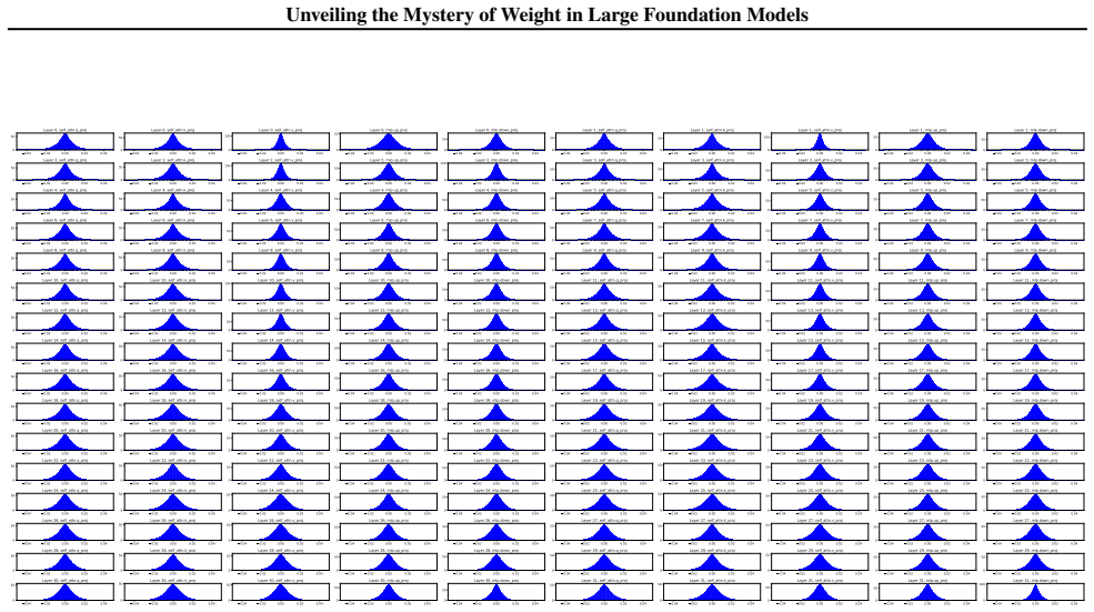
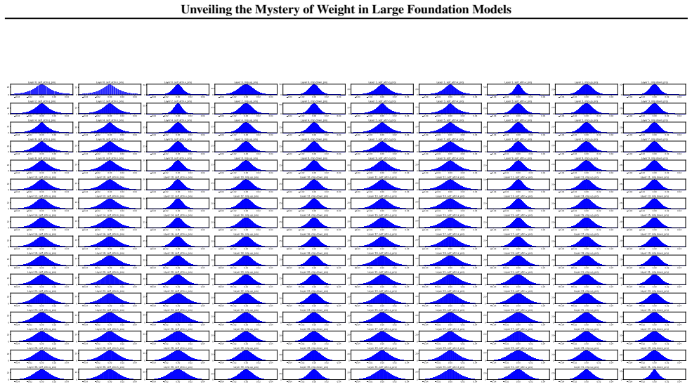
On the paper's own terms, the central discovery is that the observed Gaussian shape of pretrained weights is not incidental but structural: the paper reports that in LLaMA, Vicuna, Qwen2.5, SAM, ConvNeXt, SigLip, Idefics3, LLaVA-NeXT, and Ovis1.6, on average over 99 percent of weight elements survive a 3σ filter, skewness is 0, and kurtosis sits near 3. Combining that marginal Gaussian with an assumed asymptotic independence of weight elements, the paper concludes the weights are i.i.d. Gaussian noise, so the difference between pretrained and fine-tuned weights should itself be pure noise with an adjustable standard deviation. It tests this by freezing a randomly initialized Gaussian matrix per layer and training only one scalar $s$ in $W' = W + s\Delta W$ on GLUE with DeBERTaV3-base, reaching a 78.62 average with 72 parameters, about 7 points above a head-only baseline. The paper further claims that this noise's standard deviation grows with layer depth, that optimal weights $W^*$ are zero-mean, symmetric, and sparse with truncated-Gaussian values and outliers, and that adaptation and merging succeed by respectively increasing σ while updating outliers and by amplifying outliers while averaging the Gaussian part; the LoRA variant and merging rule built from these claims beat their baselines by up to 7.8 and 2.0 points.
Load-bearing premise
The paper's Gaussian-noise interpretation rests on the borrowed premise that individual weight elements inside a trained matrix are asymptotically independent; if elements are actually correlated, the step from 'the histogram is Gaussian' to 'the weights are i.i.d. Gaussian noise' fails and the derivation behind the scalar-only method collapses.
Editorial extensions
If this is right
- Fine-tuning a pretrained layer can be approximated per layer by a scalar: augmenting LoRA with a Gaussian term and learning only the scale lifts commonsense-reasoning accuracy by up to 7.8 points over LoRA alone on LLaMA2-7B.
- Because the standard deviation of the transformation weights grows with layer depth, adaptation effort should concentrate on deeper layers, and per-layer σ becomes a natural budget for where to spend parameters.
- Model merging should preserve outliers beyond $t\sigma$ and average the Gaussian remainder; this rule beats plain weight averaging by 2.0 points on a multimodal benchmark.
- The learned scalar $s$ in the Gaussian-noise experiment is stable across random seeds (average difference 0.009), implying the standard deviation, not the specific noise draw, carries the adaptation signal.
- The paper's sigma-based evaluation conjecture, if confirmed, would let practitioners rank fine-tuning methods by comparing the standard deviations of their weight changes without running a test set.
Reading between the lines
- If per-layer σ truly encodes adaptation, then hyperparameters like rank and learning rate should be predictable from σ alone; a cheap test is to train any PEFT method, record its layer-wise σ, and check whether it predicts that method's accuracy across a grid of configurations.
- The sharp, inverted-T, and linear weight patterns in shallow layers are read by the paper as small-noise windows onto the sparse $W^*$; a testable extension is to use per-layer kurtosis as a proxy for training quality or layer difficulty.
- The i.i.d. assumption is the natural place to probe: measuring the correlation spectrum of attention projections would either harden the foundation or, if correlations are strong, reduce the paper's contribution to an empirical heuristic that still works.
- The sigma-gap versus performance-gap hypothesis could be stress-tested across many methods and seeds on one task, plotting $|\sigma_1 - \sigma_2|$ against accuracy difference; the paper itself calls this only preliminarily validated.
Editorial analysis
A structured set of objections, weighed in public.
Referee Report
Summary. The paper claims that pretrained and fine-tuned weight matrices of large foundation models are predominantly Gaussian, that weight elements are i.i.d. like Gaussian noise, that transformation weights can be replaced by Gaussian noise with a learned scalar standard deviation, and that the underlying optimal weights are zero-mean, symmetric, and sparse with truncated Gaussian entries plus outliers. It then proposes two applications: LoRA+Ours, which augments LoRA by also learning a scalar multiplier of the pretrained weight matrix, and a model-merging method that amplifies outliers outside a per-layer threshold. The empirical sections report consistent improvements in commonsense reasoning (up to +7.8 points over LoRA) and in multimodal model merging (+2.0 points over averaging).
Significance. The empirical portion of the paper is valuable: the observation that a randomly initialized Gaussian Delta-W with a single learned scalar per layer recovers a large fraction of full fine-tuning performance on GLUE (Table 2) is a striking and falsifiable result, and the proposed LoRA+Ours and merging methods give clear gains. The paper also documents weight histograms across nine models in NLP, CV, and MM, which could serve as a useful reference. However, the theoretical framing goes well beyond what the evidence supports. The i.i.d. claim rests on an unverified independence assumption, the Gaussianity validation uses post hoc filtering, and the M-estimator derivation of W* contains unjustified structural assumptions and a mathematical error in the variance algebra. The paper would be significantly improved by reframing the theoretical claims as conjectures and adding direct tests of independence and distributional fit.
major comments (5)
- [Sec. 3.1, Eq. (1)] The derivation of the i.i.d. property assumes independence rather than establishing it. Eq. (1) writes the joint density as a product of Gaussians after noting that the observed pooled histogram is approximately Gaussian, but a Gaussian marginal for the pooled entries does not imply that the entries are independent or identically distributed. The cited references address initialization or random-matrix limits, not trained transformer weights. Since the subsequent claim that transformation weights can be 'directly derived from Gaussian noise' depends on this i.i.d. interpretation, the paper needs either a direct test of independence (e.g., correlation or autocorrelation statistics on the weight matrices) or a reformulation that does not claim i.i.d. properties.
- [Appendix A.2, Eq. (8)] The variance algebra in Eq. (8) is incorrect as written. If W and W' are independent samples from distributions with variances sigma_1^2/n and sigma_2^2/m, then the variance of their difference Delta-W is the sum of the two variances, not the difference. If they are correlated because both share W*, then a covariance term is required. The expression 'sigma_2^2/m - sigma_1^2/n' can even be negative, which is impossible for a variance. This error undermines the derivation that Delta-W is zero-mean Gaussian with variance equal to the difference of the two noise variances, which is then used in Sec. 3.3 to explain why adding Gaussian noise helps.
- [Sec. 2.2 and Appendix A.1, Table 5] The Gaussianity claim is weakened by post hoc filtering. The main validation computes skewness and kurtosis only after a 3-sigma filter, and Appendix A.1 shows that for layers with high kurtosis (e.g., 3.7-4.5 in ConvNeXt-xlarge stage 2), kurtosis drops to about 3 only after additionally removing all values with magnitude below 10^-3. The ratio reported in Table 1 (99%+) corresponds to the 3-sigma filter only, so the reader has no sense of how much data is removed by the second filter. This does not support the blanket statement that 'nearly all pre-trained weights conform to a Gaussian distribution.' The authors should report the full filtering procedure and the retained fraction for both filters, or use a distributional test on unfiltered weights.
- [Sec. 3.3, Eqs. (4)-(5)] The M-estimator argument treats the entire pretrained weight vector as a finite-dimensional parameter estimated from n i.i.d. samples and concludes that W - W* is asymptotically normal with isotropic covariance sigma^2 I. This is an assumption, not a derivation. Neural network weights are high-dimensional and trained with SGD on non-i.i.d. data, and no justification is given for the spherical covariance or for the applicability of classical M-estimator asymptotics to this setting. The subsequent interpretation of W as W* plus Gaussian noise, and the properties of W* derived in Sec. 4, inherit this unverified assumption. The authors should either provide a rigorous argument or explicitly label this as a heuristic model.
- [Appendix B.2] The simulation in Appendix B.2 is a curve-fitting exercise, not an independent validation of the W* hypothesis. The standard deviations of the added Gaussian noise (0.001 to 0.3), the truncation bounds (0.001 and 0.5), the sparsity (2 million nonzero of 10 million), and the outlier fraction (0.5% in [0.6, 1]) are all selected after observing the target histograms. The paper even acknowledges in Appendix B that W* is unverifiable. The conclusion that the observed distributions 'can be derived' from the hypothesized W* therefore has no falsifiable content. The authors should soften the claim to a demonstration of plausibility, or propose a concrete, testable implication of the W* model that goes beyond reproducing the already-observed shapes.
minor comments (6)
- [Title] The title in the PDF body reads 'Gaussian Distribution Never F ades' with an erroneous space; this should be corrected to 'Fades'.
- [Sec. 2.2] There is a typo in the sentence 'kurtosis describes the "tailedness" of a it'; it should read 'of a distribution'.
- [Sec. 3.2] The narrative moves from 'carefully crafted Delta-W matrices' that use auxiliary information from fully fine-tuned weights to 'randomly initialized with standard Gaussian noise' without clearly distinguishing the two experimental protocols. The transition should be made explicit so the reader understands that the Gaussian-noise result is a separate ablation.
- [Sec. 4] The phrase 'This comes to the conflict' should be 'This leads to a conflict' or 'This creates a conflict'.
- [Table 4] The table formatting is broken: the line '36.9Math-LLaV A' concatenates the average score for LLaVA-1.6-13B with the model name for Math-LLaVA. The table should be reformatted for clarity.
- [Appendix B.2] The final sentence 'For experimental details, please refer to Appendix. B.2.' refers to the section in which it appears; the intended cross-reference is presumably Appendix C.6.
Circularity Check
Partial circularity: the W*-hypothesis 'validation' and the ΔW-Gaussianity derivation reduce to their own assumptions, while the direct histogram observations remain independent.
-
fitted input called prediction
[Appendix B.2, Fig. 7; simulation parameters in Appendix C.6]
"We first simulate W∗. We randomly fit a sparse matrix and assign its values a truncated Gaussian distribution. Specifically, we set the standard deviation of the Gaussian distribution to 0.1, and then filter out values whose absolute values are less than 0.001 or greater than 0.5, resulting in a truncated Gaussian distribution. Next, we simulate the training process by adding different levels of Gaussian noise to W∗. ... Therefore, based on the properties of W∗, we have derived the weight distributions under various conditions, which correspond well to the observed cases."
The observed distribution shapes (linear, inverted T, sharp, Gaussian) are produced by explicitly assuming the hypothesis under test: W∗ is a sparse truncated Gaussian plus outliers, and observed weights are W∗ plus Gaussian noise. The noise levels (0.001 to 0.3), truncation bounds (0.001 and 0.5), sparsity ratio (20%), outlier fraction (0.5%), and outlier magnitudes ([0.6, 1]) are hand-chosen in Appendix C.6 to reproduce the target shapes. Figure 7 is therefore a fit of the hypothesis to the data, not an independent derivation or prediction. The paper labels this 'derivation' and 'validation,' but the match is by construction because the simulation's inputs already encode the conclusion it claims to support.
-
other
[Appendix A.2, Eqs. (7)-(8)]
"Through observation, we know that both the pretrained weights and the fine-tuned weights follow a Gaussian distribution. Naturally, since the transformation weights are the difference between these two sets of weights, they too should follow a Gaussian distribution. ... This implies that ∆W follows a Gaussian distribution with a mean of 0."
Equation (7) begins by assuming W = W∗ + N(0, σ1²/n I) and W′ = W∗ + N(0, σ2²/m I), i.e., it assumes exactly the Gaussian-noise characterization of weights that the paper claims to establish. The conclusion that ΔW is Gaussian then follows formally as the difference of two Gaussian terms, so Eq. (8) restates the model rather than independently deriving the observed Gaussianity of transformation weights. The paper presents this as explaining why 'transformation weights can be directly derived from Gaussian noise,' but the premise already contains that conclusion; the empirical observation is only the histogram shape, which the derivation does not independently produce.
full rationale
The paper's primary observational claims — that pretrained and fine-tuned weight histograms are approximately Gaussian, with near-zero skewness and kurtosis near 3 — are direct measurements and are not circular. The Sec. 3.2 experiment, in which a random Gaussian ΔW with a trained per-layer scalar s achieves nontrivial GLUE performance, is also genuine empirical evidence with real predictive content. The circularity is partial and located in two places. First, the Appendix B.2 simulation purports to 'derive' the observed distributions from the hypothesized optimal weights W∗, but it constructs W∗ and the additive Gaussian noise using parameters chosen to reproduce those same distributions, making the agreement a fit rather than a validation. Second, the derivation of ΔW's Gaussianity in Appendix A.2 assumes Eq. (7), which already encodes the Gaussian-noise model for W and W′, so Eq. (8) is a tautological consequence, not an independent first-principles derivation. Additionally, the i.i.d. conclusion in Sec. 3.1 depends on a borrowed and unverified premise — asymptotic independence of individual weight elements, cited to initialization and random-matrix literature — and the paper provides no correlation tests; this is a load-bearing missing-support issue rather than a circularity per se. Self-citations (Si et al. 2024a,b,c) are used as method baselines and PEFT references, not to establish the Gaussian claim, so they do not increase the circularity score. Overall, the direct histogram observations remain independent, but two claimed derivations/validations reduce to their own inputs, giving a partial circularity score of 6.
Assumptions & free parameters
free parameters (6)
- W* simulation Gaussian sigma =
0.1
- W* truncation bounds =
[-0.5, -0.001] union [0.001, 0.5]
- Simulated sparsity =
20% (2M of 10M nonzero)
- Simulated outlier fraction and range =
0.5% of nonzero in [0.6, 1]
- Validation filter thresholds =
3-sigma filter plus 10^-3 small-value filter
- Merging threshold multiplier t =
2 and 3 (best reported t=2)
assumptions (7)
- domain assumption Individual weight elements are asymptotically independent
- standard math The trained weight matrix W is an M-estimator of an optimal W* with sqrt(n)(W-W*) converging to N(0, sigma^2 I)
- ad hoc to paper The asymptotic covariance of W is isotropic (sigma^2 I)
- domain assumption Pre-training and fine-tuning datasets are subsets of the dataset defining W*
- domain assumption Training injects zero-mean Gaussian noise with layer-dependent variance
- domain assumption Shallow layers are easier to train and thus closer to W*
- ad hoc to paper Occam's razor and simplicity principles constrain the form of W*
invented entities (1)
-
Optimal weight matrix W*
Cite this review
Pith. "Pith review of Unveiling the Mystery of Weight in Large Foundation Models: Gaussian Distribution Never Fades." pith.science (2026). https://pith.science/paper/MJZLP5RZ
@misc{pith2026250110661,
  author       = {Pith},
  title        = {Pith review of: Unveiling the Mystery of Weight in Large Foundation Models: Gaussian Distribution Never Fades},
  year         = {2026},
  howpublished = {\url{https://pith.science/paper/MJZLP5RZ}},
  note         = {Machine review of arXiv:2501.10661}
}
read the original abstract
This paper presents a pioneering exploration of the mechanisms underlying large foundation models' (LFMs) weights, aiming to simplify AI research. Through extensive observation and analysis on prevailing LFMs, we find that regardless of initialization strategies, their weights predominantly follow a Gaussian distribution, with occasional sharp, inverted T-shaped, or linear patterns. We further discover that the weights share the i.i.d. properties of Gaussian noise, and explore their direct relationship. We find that transformation weights can be derived from Gaussian noise, and they primarily serve to increase the standard deviation of pre-trained weights, with their standard deviation growing with layer depth. In other words, transformation weights broaden the acceptable deviation from the optimal weights, facilitating adaptation to downstream tasks. Building upon the above conclusions, we thoroughly discussed the nature of optimal weights, ultimately concluding that they should exhibit zero-mean, symmetry, and sparsity, with the sparse values being a truncated Gaussian distribution and a few outliers. Our experiments in LFM adaptation and editing demonstrate the effectiveness of these insights. We hope these findings can provide a foundational understanding to pave the way for future advancements in the LFM community.
Figures


Figures from the paper (23 more)





Forward citations
Cited by 1 Pith paper
-
NAN: A Training-Free Solution to Coefficient Estimation in Model Merging
NAN sets merging coefficients inversely proportional to each model's parameter norm and claims a least-squares justification, but the derivation yields a different formula and performance gains are inconsistent.
Reference graph
Works this paper leans on
-
[1]
A): We provide a more in-depth exploration of weight distribution
Exploration of Weight Distribution (Appendix. A): We provide a more in-depth exploration of weight distribution
-
[2]
B): Here, we delve deeper into the discussion of W∗
Open Discussion (Appendix. B): Here, we delve deeper into the discussion of W∗. We strongly encourage readers to review this section for a more profound understanding of our work
-
[3]
C): We include all experimental details presented in the main text
Experimental Details (Appendix. C): We include all experimental details presented in the main text
-
[4]
D): Other supplementary information, such as algorithm tables, will also be provided
Additional Details (Appendix. D): Other supplementary information, such as algorithm tables, will also be provided
-
[5]
E): We will introduce relevant literature related to our work
Related Work (Appendix. E): We will introduce relevant literature related to our work
-
[6]
Weight Distribution Plots: We will supplement the appendix with weight distribution plots for all layers of the model. We hope that the researchers could have a happy journey, and we hope that after reviewing the appendix, they will gain a deeper understanding of our entire work. Contributions The contributions of this paper are as follows: • We conducted...
-
[12]
Transformation Weights Follow a Gaussian Distribution: 17 Unveiling the Mystery of Weight in Large Foundation Models We have not dedicated much effort to elaborating on the fact that the transformation follows a Gaussian distribution, since we think it is natural for the following reasons. Through observation, we know that both the pretrained weights and ...
-
[13]
Here, we also validate ∆W obtained from LoRA-Dash and DoRA
Gaussian Noise in Transformation Weights Complements the Standard Deviation of That in Pre-training: Additionally, in the paper, we mention that the Gaussian noise in ∆W serves to complement the standard deviation of the Gaussian noise in pre-training. Here, we also validate ∆W obtained from LoRA-Dash and DoRA. We first present the results of these two me...
work page 2019
Show all 16 references
-
[14]
The results are shown in the Table
The Closer the Standard Deviations of Two ∆W, the More Similar the Corresponding Model Performance Becomes: Furthermore, we compared the differences in the standard deviations of ∆W obtained from LoRA-Dash and DoRA for the same rank. The results are shown in the Table. 7, row ...
-
[15]
physical experiment
The Standard Deviation of ∆W Increases with the Layer Depth: As will be shown in Appendix. B, the Gaussian noise introduced during the training of each layer increases as the layer depth 17Given that the performance of DoRA at r = 4 is significantly lower, we exclude this sett...
2002
-
[204]
Clark, C., Lee, K., Chang, M.-W., Kwiatkowski, T., Collins, M., and Toutanova, K
PMLR, 2015. Clark, C., Lee, K., Chang, M.-W., Kwiatkowski, T., Collins, M., and Toutanova, K. Boolq: Exploring the surprising difficulty of natural yes/no questions. arXiv preprint arXiv:1905.10044, 2019. Clark, P., Cowhey, I., Etzioni, O., Khot, T., Sabharwal, A., Schoenick, ...
2015 arXiv
-
[645]
He, M., Liu, Y ., Wu, B., Yuan, J., Wang, Y ., Huang, T., and Zhao, B
Springer, 2016b. He, M., Liu, Y ., Wu, B., Yuan, J., Wang, Y ., Huang, T., and Zhao, B. Efficient multimodal learning from data-centric perspective. arXiv preprint arXiv:2402.11530, 2024. He, P., Gao, J., and Chen, W. Debertav3: Im- proving deberta using electra-style pre-trai...
2024 arXiv
-
[1126]
Feng, T., Jin, C., Liu, J., Zhu, K., Tu, H., Cheng, Z., Lin, G., and You, J
IOS Press, 2020. Feng, T., Jin, C., Liu, J., Zhu, K., Tu, H., Cheng, Z., Lin, G., and You, J. How far are we from agi. arXiv preprint arXiv:2405.10313, 2024. Fischer, M., Bartler, A., and Yang, B. Prompt tuning for parameter-efficient medical image segmentation.Medical Image A...
2020 arXiv
-
[2023]
However, existing studies have rarely validated or analyzed these observations in depth
noted that trained weights often exhibit Gaussian-like patterns. However, existing studies have rarely validated or analyzed these observations in depth. Most works have either mentioned Gaussian properties in passing or treated them as incidental findings without further expl...
2023
-
[2799]
PMLR, 2019. Hu, E. J., Shen, Y ., Wallis, P., Allen-Zhu, Z., Li, Y ., Wang, S., Wang, L., and Chen, W. Lora: Low-rank adaptation of large language models. arXiv preprint arXiv:2106.09685, 2021. Hu, Z., Wang, L., Lan, Y ., Xu, W., Lim, E.-P., Bing, L., Xu, X., Poria, S., and Le...
2019 arXiv
-
[3938]
10 Unveiling the Mystery of Weight in Large Foundation Models Han, K., Wang, Y ., Chen, H., Chen, X., Guo, J., Liu, Z., Tang, Y ., Xiao, A., Xu, C., Xu, Y ., et al
PMLR, 2020. 10 Unveiling the Mystery of Weight in Large Foundation Models Han, K., Wang, Y ., Chen, H., Chen, X., Guo, J., Liu, Z., Tang, Y ., Xiao, A., Xu, C., Xu, Y ., et al. A survey on vision transformer. IEEE transactions on pattern analysis and machine intelligence, 45(1...
2020 arXiv
Reviewed August 10, 2026 · model on record in the stance chip above.
Discussion (0). Continue with ORCID to comment.