REVIEW 4 major objections 6 minor 41 references
GeomGS: LiDAR-Guided Geometry-Aware Gaussian Splatting for Robot Localization
T0 review · 4 major / 6 minor · reviewed 2026-08-10 · deepseek-v4-flash
Pith's one-line read Adding a Geometric Confidence Score to LiDAR-seeded Gaussian splatting yields metric-scale maps accurate enough for scan-plus-image robot localization.
desk verdict The localization evaluation is circular—query scans come from the same 100 frames used to build the map—so the headline accuracy numbers measure self-registration, not localization. read the letter →
The pith
A machine-rendered reading of the paper's core claim, the machinery that carries it, and where it could break.
The reading
What carries the argument
The load-bearing object is the Geometric Confidence Score $\gamma \in (0,1)$, computed toward an asymmetric sigmoid $\sigma_{\mathrm{asym}}(x) = 1/(1+e^{k(x-d)})$ with $k=20$ and $d=0.9$, where $x$ is the distance $d_i = \min_{p\in P}\|g_i-p\|_2$ from Gaussian $g_i$ to the accumulated LiDAR prior $P$. Two losses carry the geometry: $\mathcal{L}_{\mathrm{geom}}$ drives $\gamma_i$ toward $\sigma_{\mathrm{asym}}(d_i)$, and $\mathcal{L}_{\mathrm{prob}}$ applies the cost $(1/N)\sum_i (\ln(1-\gamma_i) + d_i/(1-\gamma_i))$, which downweights Gaussians that exist mainly for rendering. The same GCS is reused at localization time as the diagonal weight matrix in weighted ICP, linking mapping quality directly to pose estimation.
What would settle it
Rebuild each map without the LiDAR scans belonging to the test frames, rerun the paper's localization protocol, and compare rotation and translation errors; if the errors grow substantially, the reported localization accuracy depends on the query scan being contained in the map.
Extended reading notes
Core claim
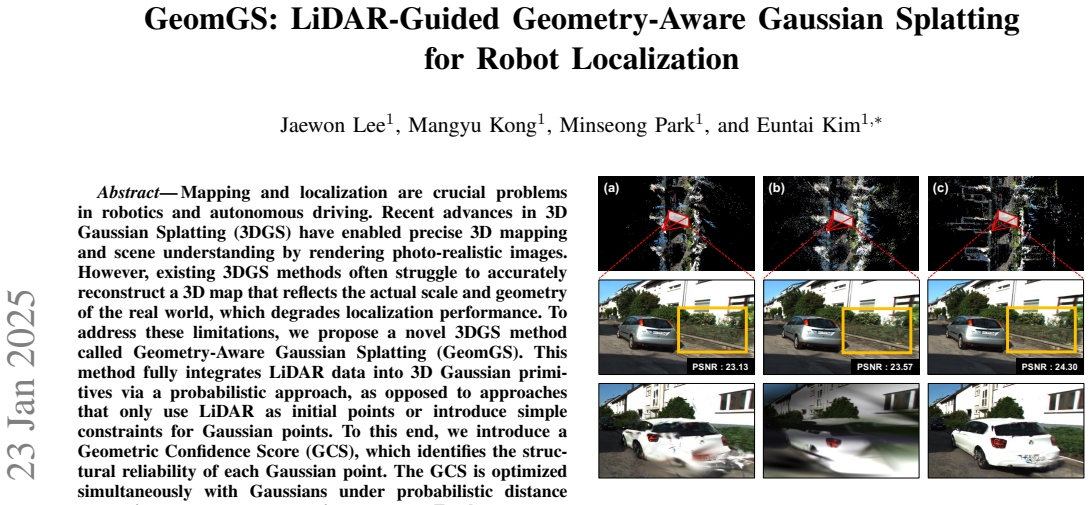
The paper's central claim is that LiDAR can be fully integrated into 3D Gaussian primitives rather than merely used as initialization or a soft pull. GeomGS introduces the Geometric Confidence Score, a per-Gaussian parameter optimized to be close to an asymmetric sigmoid of the distance to the nearest accumulated LiDAR point, and a probabilistic distance loss that assigns higher weight to high-confidence Gaussians. The result is claimed to be a map that preserves metric scale and structure without sacrificing photometric quality. On that map the paper proposes a localization pipeline in which a query LiDAR scan is aligned by weighted ICP using GCS as per-point weights, the pose is then refined by minimizing the photometric error between a rendered image and the query image, and the two steps are iterated. Across its urban-driving benchmarks, the paper reports the lowest Chamfer distance and highest F-score among the compared methods, improved PSNR/SSIM/LPIPS relative to the baselines it compares, and lower rotation and translation errors than plain ICP, weighted ICP alone, or image-only refinement.
Load-bearing premise
The evaluation's load-bearing premise is that the every-10th query scan is not part of the accumulated LiDAR prior P; the paper never states this exclusion, so the reported localization errors may measure alignment to a map containing the query's own points.
Editorial extensions
If this is right
- Maps produced by GeomGS carry metric scale and structural detail, so downstream robotics tasks that need true geometry, not just pretty rendering, can use them directly.
- The same per-point confidence map that guides mapping also serves as ICP weighting, so geometric reliability discovered during mapping transfers to localization without extra learned components.
- Alternating weighted scan alignment with image-based refinement covers each method's failure mode: image refinement corrects scan misalignment, while scan alignment fixes large pose errors that image-only refinement misses.
- Because the geometry losses only pull high-confidence Gaussians toward LiDAR, regions such as sky and tall buildings can remain rendering-oriented without distorting the surveyed structure.
Reading between the lines
- The paper's localization protocol selects every 10th of 100 frames as test cases but never states that these frames are excluded from the accumulated LiDAR prior built over all poses; if they are included, the reported errors partly measure registration to the query's own points rather than localization within an unseen map.
- A natural test the paper does not run is to rebuild the map from the remaining 90 scans and repeat the localization table; that would quantify how much of the claimed accuracy survives genuine map novelty.
- The GCS could be exported beyond localization, for example as a reliability mask for pruning unstable Gaussians or for detecting changed regions in a revisited scene.
- The probabilistic distance loss's behavior under denser or noisier LiDAR is untested; perturbing the input scans would show whether the structural gains persist across sensor characteristics.
Editorial analysis
A structured set of objections, weighed in public.
Referee Report
Summary. The paper proposes GeomGS, a 3D Gaussian Splatting variant that initializes Gaussians from accumulated LiDAR point clouds and introduces a per-Gaussian Geometric Confidence Score (GCS). GCS is fitted to an asymmetric sigmoid of the distance to the nearest LiDAR point and is used to reweight a probabilistic distance loss. A localization module alternates GCS-weighted ICP against the Gaussian map with iNeRF-style image refinement. Experiments on KITTI and KITTI-360 report image quality, geometric fidelity, and localization accuracy.
Significance. Accurate metric-scale maps for localization are a relevant problem, and combining LiDAR priors with 3DGS is timely. The paper presents a concrete system with comparisons to several 3DGS variants and a localization pipeline that integrates LiDAR and photometric cues. However, the evaluation protocol as described does not establish the claimed state-of-the-art localization or geometric accuracy, because the query LiDAR scans and test images appear to be part of the mapping set. If the method were re-evaluated on a genuinely held-out split, the underlying idea of GCS-weighted ICP with image refinement could still be of interest, but the central claims currently rest on an evaluation that measures self-registration rather than generalization.
major comments (4)
- [Section IV-A/IV-D, Table III] The localization evaluation is circular. Mapping uses 100 consecutive images and builds the accumulated LiDAR prior P = union_i (T_i P_i) from the poses of those images (Eq. 5). Section IV-D then selects test cases from every 10th sequence out of those 100 sequences without stating that those sequences are excluded from mapping. Under the natural reading, each query scan Q_p is a subset of P, so the weighted ICP (Eqs. 14-16) aligns the query to a map that already contains the query's own points. The errors in Table III therefore measure self-registration, not localization against an unseen map. The image-refinement stage has the same problem if the query images are among the images used to train the photometric loss. Please re-run the evaluation with a held-out split, such as a separate sequence or temporally disjoint scans, and report exactly which frames and scans are used for mapping versus testing.
- [Section IV-C, Table II] The geometric quality metrics in Table II are computed between the optimized Gaussians G and the accumulated LiDAR points P, which is the very target used in the distance losses L_geom and L_prob (Eqs. 7-9). A method that is explicitly constrained to move Gaussians toward P will trivially score well on Chamfer distance and F-score against P. This does not demonstrate that the map is geometrically accurate in an independent sense; it only shows that the constraint was enforced. Please evaluate against held-out LiDAR scans, a ground-truth mesh, or at least a separate validation LiDAR scan that was not used in mapping.
- [Section III-B, Eqs. (6)-(9)] The GCS is not learned from an independent geometric signal: Eq. 8 fits gamma_i to a hand-set asymmetric sigmoid of d_i, and Eq. 9 then uses gamma_i to reweight the same d_i in the distance loss. As written, the 'probabilistic distance constraint' is a deterministic reweighting of the nearest-neighbor distance by a fixed function of that distance. The paper should clarify what is actually learned beyond the hand-set sigmoid parameters k and d, and justify why this constitutes a probabilistic model rather than a heuristic robust weighting. If the intended contribution is only a heuristic weighting, the terms 'probabilistic' and 'Geometric Confidence Score' as a learned parameter should be revised accordingly.
- [Section IV-B, Table I] The image-quality evaluation is described as 'testing on scenes sampled every 8 frames' from the same 100-frame sequence used for mapping, with no statement that these frames are held out during training. If the training set includes all 100 frames, the PSNR/SSIM/LPIPS results in Table I are self-reconstruction scores rather than novel-view synthesis results. Please specify the exact training/test image split and, if the current protocol does not hold out test frames, retrain on the remaining frames and report the corresponding numbers.
minor comments (6)
- [Throughout] There are several typos and formatting errors, including 'QUANTITAIVE' in Table I, 'PERFORMACE' in Table II, and the footnote '∗is that the corresponding author' in Section I.
- [Eq. (10)] In Eq. (10), the L1 term uses I_a (appearance-model image) while the SSIM term uses I_r (rendered image); it would be clearer to state whether the L1 loss is intentionally computed against the appearance-model output rather than the standard rendered image.
- [Eq. (14)] In Eq. (14), W = diag(gamma) uses GCS values, but it is not specified whether these weights are applied to the source (query LiDAR) points, the target (Gaussian map) points, or both; since the query scan has no GCS, the intended construction of S, T, and W should be stated explicitly.
- [Section IV-A] The paper uses both '100 consecutive images' and 'every 10th sequence out of 100 sequences'; it should clarify whether a 'sequence' is a single frame or a sub-sequence, since this affects the number of localization test cases.
- [Table III] No standard deviations or number of runs are reported for the localization experiments, so it is unclear whether the differences between methods are statistically significant.
- [References] Some references are incomplete or inconsistently formatted, such as [33] (missing venue) and [34] (arXiv preprint without a clear publication status).
Circularity Check
Localization and geometry evaluations are circular: query scans are drawn from the same 100-frame set used to build the LiDAR prior P, so WICP aligns each query to its own points, and CD/F-Score compare the Gaussians to the very P used as supervision.
-
fitted input called prediction
[Section III-B (Eq. 5); Section IV-A; Section IV-D; Table III]
"The transformed LiDAR scans from all poses are then combined into the final accumulated point cloud P, as shown in Eq. 5: P = ∪_i (T_i P_i). ... We selected 100 consecutive images from KITTI [38] and KITTI-360 [39] datasets ... For the evaluation, we selected test cases from every 10th sequence out of 100 sequences and calculated the average localization performance."
The accumulated LiDAR prior P is built from the LiDAR scans of all poses in the 100-frame mapping set (Eq. 5). The localization evaluation then takes query test cases from every 10th sequence of those same 100 sequences, with no statement that these frames were excluded from the map. Under the natural reading, each query scan Q_p is one of the P_i already contained in P, so the Weighted ICP step (Eqs. 14-16) registers Q_p to a map that contains Q_p's own points. The rotation/translation errors in Table III therefore measure self-alignment, not localization against an unseen map; the photometric refinement likewise uses training views from L_rgb (Eq. 10).
-
self definitional
[Section III-B (Eqs. 7-9); Section IV-C (Eqs. 17-19); Table II]
"di = min p∈P ∥gi − p∥2, gi ∈ G ... Lprob = 1/N Σ (ln(1 − γi) + di/(1 − γi)) ... we calculate Chamfer Distance (CD), as shown in Eq. 17, and the F-Score, as shown in Eq. 19. We then compare these metrics between the generated Gaussians G and the accumulated LiDAR Points P."
The probabilistic loss Lprob directly penalizes d_i, the distance from each Gaussian to the accumulated LiDAR point cloud P (Eq. 7). The geometric validation then computes Chamfer Distance and F-Score between the same G and the same P (Section IV-C). The metrics in Table II therefore measure how well the optimization minimized its own supervision target; they are not an independent assessment of geometric accuracy. The claim of state-of-the-art geometric performance reduces by construction to a restatement of the fitting objective.
full rationale
Score 8: the paper's headline claims of geometric and localization superiority are supported by evaluations that reduce, by construction, to the method's own supervision. The localization protocol (Sections IV-A and IV-D) never states that query frames are excluded from the 100-frame mapping set; since Eq. 5 builds the LiDAR prior P from the transformed scans of all poses, the Weighted ICP in Table III aligns each query scan to a map containing that exact scan, and the image refinement uses the corresponding training views. Independently, the geometric metrics in Table II compare the Gaussians to the same accumulated LiDAR points P that Eq. 9 uses as the target of Lprob, so the high F-Score/low CD is a fit diagnostic rather than an external benchmark. The GCS reweighting (Eqs. 6, 8, 9) is also an internal transformation of the same distance d_i rather than an independent signal, but the decisive circularity is the evaluation design. No self-citation chain is load-bearing. If a held-out split was intended, the paper does not describe it; as written, the central claims are not supported.
Assumptions & free parameters
free parameters (8)
- GCS sigmoid slope k =
20
- GCS sigmoid dividing point d =
0.9
- Loss weight lambda_rgb =
0.2
- Loss weight lambda_geom =
0.1
- Loss weight lambda_prob =
0.1
- Loss weight lambda_scale =
100.0
- Loss weight lambda_perc =
0.5
- Initial position learning rate =
1.6e-5
assumptions (3)
- domain assumption The accumulated LiDAR point cloud P (Eq. 5) is an accurate geometric ground truth and a valid localization target.
- ad hoc to paper The asymmetric sigmoid form of GCS (Eq. 6) with hand-set k and d is a valid confidence model.
- domain assumption Eq. 9 is a probabilistic distance constraint as claimed, inherited from [8].
invented entities (1)
-
Geometric Confidence Score (GCS) gamma
Cite this review
Pith. "Pith review of GeomGS: LiDAR-Guided Geometry-Aware Gaussian Splatting for Robot Localization." pith.science (2026). https://pith.science/paper/CX6FNGTU
@misc{pith2026250113417,
  author       = {Pith},
  title        = {Pith review of: GeomGS: LiDAR-Guided Geometry-Aware Gaussian Splatting for Robot Localization},
  year         = {2026},
  howpublished = {\url{https://pith.science/paper/CX6FNGTU}},
  note         = {Machine review of arXiv:2501.13417}
}
read the original abstract
Mapping and localization are crucial problems in robotics and autonomous driving. Recent advances in 3D Gaussian Splatting (3DGS) have enabled precise 3D mapping and scene understanding by rendering photo-realistic images. However, existing 3DGS methods often struggle to accurately reconstruct a 3D map that reflects the actual scale and geometry of the real world, which degrades localization performance. To address these limitations, we propose a novel 3DGS method called Geometry-Aware Gaussian Splatting (GeomGS). This method fully integrates LiDAR data into 3D Gaussian primitives via a probabilistic approach, as opposed to approaches that only use LiDAR as initial points or introduce simple constraints for Gaussian points. To this end, we introduce a Geometric Confidence Score (GCS), which identifies the structural reliability of each Gaussian point. The GCS is optimized simultaneously with Gaussians under probabilistic distance constraints to construct a precise structure. Furthermore, we propose a novel localization method that fully utilizes both the geometric and photometric properties of GeomGS. Our GeomGS demonstrates state-of-the-art geometric and localization performance across several benchmarks, while also improving photometric performance.
Figures


Figures from the paper (1 more)

Reference graph
Works this paper leans on
-
[1]
Structure-from-motion revisited,
J. L. Sch ¨onberger and J.-M. Frahm, “Structure-from-motion revisited,” in Conference on Computer Vision and Pattern Recognition (CVPR) , 2016
2016
-
[2]
Scaffold-gs: Structured 3d gaussians for view-adaptive rendering,
T. Lu, M. Yu, L. Xu, Y . Xiangli, L. Wang, D. Lin, and B. Dai, “Scaffold-gs: Structured 3d gaussians for view-adaptive rendering,” in Proceedings of the IEEE/CVF Conference on Computer Vision and Pattern Recognition, 2024, pp. 20 654–20 664
2024
-
[3]
J. Li, J. Zhang, X. Bai, J. Zheng, X. Ning, J. Zhou, and L. Gu, “Dngaussian: Optimizing sparse-view 3d gaussian radiance fields with global-local depth normalization,” in Proceedings of the IEEE/CVF Conference on Computer Vision and Pattern Recognition , 2024, pp. 20 775–20 785
work page 2024
-
[4]
Street gaussians: Modeling dynamic urban scenes with gaussian splatting,
Y . Yan, H. Lin, C. Zhou, W. Wang, H. Sun, K. Zhan, X. Lang, X. Zhou, and S. Peng, “Street gaussians: Modeling dynamic urban scenes with gaussian splatting,” in ECCV, 2024
2024
-
[5]
Vegs: View extrapolation of urban scenes in 3d gaussian splatting using learned priors,
S. Hwang, M.-J. Kim, T. Kang, J. Kang, and J. Choo, “Vegs: View extrapolation of urban scenes in 3d gaussian splatting using learned priors,” in ECCV, 2024
work page 2024
-
[6]
Colmap-free 3d gaussian splatting,
Y . Fu, S. Liu, A. Kulkarni, J. Kautz, A. A. Efros, and X. Wang, “Colmap-free 3d gaussian splatting,” in Proceedings of the IEEE/CVF Conference on Computer Vision and Pattern Recognition (CVPR), June 2024, pp. 20 796–20 805
work page 2024
-
[7]
Drivinggaussian: Composite gaussian splatting for surrounding dy- namic autonomous driving scenes,
X. Zhou, Z. Lin, X. Shan, Y . Wang, D. Sun, and M.-H. Yang, “Drivinggaussian: Composite gaussian splatting for surrounding dy- namic autonomous driving scenes,” in Proceedings of the IEEE/CVF Conference on Computer Vision and Pattern Recognition , 2024, pp. 21 634–21 643
work page 2024
-
[8]
Robust 6d object pose estimation by learning rgb-d features,
M. Tian, L. Pan, M. H. Ang, and G. H. Lee, “Robust 6d object pose estimation by learning rgb-d features,” in 2020 IEEE International Conference on Robotics and Automation (ICRA) . IEEE, 2020, pp. 6218–6224
work page 2020
Show all 41 references
-
[9]
A method for registration of 3-d shapes,
P. Besl and N. D. McKay, “A method for registration of 3-d shapes,” IEEE Transactions on Pattern Analysis and Machine Intelligence , vol. 14, no. 2, pp. 239–256, 1992
1992
-
[10]
Nerf: Representing scenes as neural radiance fields for view synthesis,
B. Mildenhall, P. P. Srinivasan, M. Tancik, J. T. Barron, R. Ramamoor- thi, and R. Ng, “Nerf: Representing scenes as neural radiance fields for view synthesis,” in ECCV, 2020
2020
-
[11]
Mip-nerf 360: Unbounded anti-aliased neural radiance fields,
J. T. Barron, B. Mildenhall, D. Verbin, P. P. Srinivasan, and P. Hedman, “Mip-nerf 360: Unbounded anti-aliased neural radiance fields,” CVPR, 2022
2022
-
[12]
Zip-nerf: Anti-aliased grid-based neural radiance fields,
J. T. Barron, B. Mildenhall, D. Verbin, P. P. Srinivasan, and P. Hed- man., “Zip-nerf: Anti-aliased grid-based neural radiance fields,” in Proceedings of the IEEE/CVF Conference on Computer Vision and Pattern Recognition, 2023, pp. 19 697–19 705
2023
-
[13]
Block-nerf: Scalable large scene neural view synthesis,
M. Tancik, V . Casser, X. Yan, S. Pradhan, B. Mildenhall, P. P. Srinivasan, J. T. Barron, and H. Kretzschmar, “Block-nerf: Scalable large scene neural view synthesis,” in Proceedings of the IEEE/CVF Conference on Computer Vision and Pattern Recognition , 2022, pp. 8248–8258
2022
-
[14]
3d gaussian splatting for real-time radiance field rendering,
B. Kerbl, G. Kopanas, T. Leimk ¨uhler, and G. Drettakis, “3d gaussian splatting for real-time radiance field rendering,” ACM Transactions on Graphics , vol. 42, no. 4, July 2023. [Online]. Available: https://repo-sam.inria.fr/fungraph/3d-gaussian-splatting/
2023
-
[15]
Dn-splatter: Depth and normal priors for gaussian splat- ting and meshing,
M. Turkulainen, X. Ren, I. Melekhov, O. Seiskari, E. Rahtu, and J. Kannala, “Dn-splatter: Depth and normal priors for gaussian splat- ting and meshing,” 2024
2024
-
[16]
Gaussianpro: 3d gaussian splatting with progressive propa- gation,
K. Cheng, X. Long, K. Yang, Y . Yao, W. Yin, Y . Ma, W. Wang, and X. Chen, “Gaussianpro: 3d gaussian splatting with progressive propa- gation,” in Forty-first International Conference on Machine Learning , 2024
2024
-
[17]
2d gaussian splatting for geometrically accurate radiance fields,
B. Huang, Z. Yu, A. Chen, A. Geiger, and S. Gao, “2d gaussian splatting for geometrically accurate radiance fields,” in SIGGRAPH 2024 Conference Papers . Association for Computing Machinery, 2024
2024
-
[18]
High-quality surface reconstruction using gaussian surfels,
P. Dai, J. Xu, W. Xie, X. Liu, H. Wang, and W. Xu, “High-quality surface reconstruction using gaussian surfels,” in ACM SIGGRAPH 2024 Conference Papers . Association for Computing Machinery, 2024
2024
-
[19]
Nerf in the wild: Neural radiance fields for unconstrained photo collections,
R. Martin-Brualla, N. Radwan, M. S. Sajjadi, J. T. Barron, A. Doso- vitskiy, and D. Duckworth, “Nerf in the wild: Neural radiance fields for unconstrained photo collections,” in Proceedings of the IEEE/CVF conference on computer vision and pattern recognition , 2021, pp. 7210–7219
2021
-
[20]
Wildgaussians: 3d gaussian splatting in the wild,
J. Kulhanek, S. Peng, Z. Kukelova, M. Pollefeys, and T. Sattler, “Wildgaussians: 3d gaussian splatting in the wild,” arXiv preprint arXiv:2407.08447, 2024
2024 arXiv
-
[21]
Vastgaussian: Vast 3d gaussians for large scene reconstruction,
J. Lin, Z. Li, X. Tang, J. Liu, S. Liu, J. Liu, Y . Lu, X. Wu, S. Xu, Y . Yan, et al. , “Vastgaussian: Vast 3d gaussians for large scene reconstruction,” in Proceedings of the IEEE/CVF Conference on Computer Vision and Pattern Recognition , 2024, pp. 5166–5175
2024
-
[22]
S-nerf: Neural radiance fields for street views,
Z. Xie, J. Zhang, W. Li, F. Zhang, and L. Zhang, “S-nerf: Neural radiance fields for street views,” in ICLR 2023, 2023
2023
-
[23]
Point-nerf: Point-based neural radiance fields,
Q. Xu, Z. Xu, J. Philip, S. Bi, Z. Shu, K. Sunkavalli, and U. Neumann, “Point-nerf: Point-based neural radiance fields,” in Proceedings of the IEEE/CVF Conference on Computer Vision and Pattern Recognition , 2022, pp. 5438–5448
2022
-
[24]
Points2nerf: Generating neural radiance fields from 3d point cloud,
D. Zimny, J. Waczy ´nska, T. Trzci ´nski, and P. Spurek, “Points2nerf: Generating neural radiance fields from 3d point cloud,” Pattern Recog- nition Letters, vol. 185, pp. 8–14, 2024
2024
-
[25]
Radsplat: Radiance field-informed gaussian splatting for robust real- time rendering with 900+ fps,
M. Niemeyer, F. Manhardt, M.-J. Rakotosaona, M. Oechsle, D. Duck- worth, R. Gosula, K. Tateno, J. Bates, D. Kaeser, and F. Tombari, “Radsplat: Radiance field-informed gaussian splatting for robust real- time rendering with 900+ fps,” arXiv.org, 2024
2024
-
[26]
Gaussiandreamer: Fast generation from text to 3d gaussians by bridging 2d and 3d diffusion models,
T. Yi, J. Fang, J. Wang, G. Wu, L. Xie, X. Zhang, W. Liu, Q. Tian, and X. Wang, “Gaussiandreamer: Fast generation from text to 3d gaussians by bridging 2d and 3d diffusion models,” in CVPR, 2024
2024
-
[27]
iNeRF: Inverting neural radiance fields for pose estimation,
L. Yen-Chen, P. Florence, J. T. Barron, A. Rodriguez, P. Isola, and T.- Y . Lin, “iNeRF: Inverting neural radiance fields for pose estimation,” in IEEE/RSJ International Conference on Intelligent Robots and Systems (IROS), 2021
2021
-
[28]
Loc-nerf: Monte carlo localization using neural radiance fields,
D. Maggio, M. Abate, J. Shi, C. Mario, and L. Carlone, “Loc-nerf: Monte carlo localization using neural radiance fields,” in 2023 IEEE International Conference on Robotics and Automation (ICRA). IEEE, 2023, pp. 4018–4025
2023
-
[29]
Fast global localization on neural radiance field,
M. Kong, S. Lee, J. Lee, and E. Kim, “Fast global localization on neural radiance field,” arXiv preprint arXiv:2406.12202 , 2024
2024 arXiv
-
[30]
Parallel inversion of neural radiance fields for robust pose estimation,
Y . Lin, T. M ¨uller, J. Tremblay, B. Wen, S. Tyree, A. Evans, P. A. Vela, and S. Birchfield, “Parallel inversion of neural radiance fields for robust pose estimation,” in 2023 IEEE International Conference on Robotics and Automation (ICRA) . IEEE, 2023, pp. 9377–9384
2023
-
[31]
Nope-nerf: Optimising neural radiance field with no pose prior,
W. Bian, Z. Wang, K. Li, J. Bian, and V . A. Prisacariu, “Nope-nerf: Optimising neural radiance field with no pose prior,” 2023
2023
-
[32]
Locndf: Neural distance field mapping for robot localization,
L. Wiesmann, T. Guadagnino, I. Vizzo, N. Zimmerman, Y . Pan, H. Kuang, J. Behley, and C. Stachniss, “Locndf: Neural distance field mapping for robot localization,” IEEE Robotics and Automation Letters, 2023
2023
-
[33]
Dreg-nerf: Deep registration for neural radi- ance fields,
Y . Chen and G. H. Lee, “Dreg-nerf: Deep registration for neural radi- ance fields,” in Proceedings of the IEEE/CVF International Conference on Computer Vision , 2023, pp. 22 703–22 713
2023
-
[34]
icomma: Inverting 3d gaussians splatting for camera pose estimation via comparing and matching,
Y . Sun, X. Wang, Y . Zhang, J. Zhang, C. Jiang, Y . Guo, and F. Wang, “icomma: Inverting 3d gaussians splatting for camera pose estimation via comparing and matching,” arXiv preprint arXiv:2312.09031, 2023
2023 arXiv
-
[35]
6dgs: 6d pose estimation from a single image and a 3d gaussian splatting model,
M. Bortolon, T. Tsesmelis, S. James, F. Poiesi, and A. Del Bue, “6dgs: 6d pose estimation from a single image and a 3d gaussian splatting model,” in ECCV, 2024
2024
-
[36]
Mixture of volumetric primitives for efficient neural rendering,
S. Lombardi, T. Simon, G. Schwartz, M. Zollhoefer, Y . Sheikh, and J. Saragih, “Mixture of volumetric primitives for efficient neural rendering,” ACM Transactions on Graphics (ToG) , vol. 40, no. 4, pp. 1–13, 2021
2021
-
[37]
Perceptual losses for real-time style transfer and super-resolution,
J. Johnson, A. Alahi, and L. Fei-Fei, “Perceptual losses for real-time style transfer and super-resolution,” in Computer Vision–ECCV 2016: 14th European Conference, Amsterdam, The Netherlands, October 11- 14, 2016, Proceedings, Part II 14 . Springer, 2016, pp. 694–711
2016
-
[38]
Are we ready for autonomous driving? the kitti vision benchmark suite,
A. Geiger, P. Lenz, and R. Urtasun, “Are we ready for autonomous driving? the kitti vision benchmark suite,” in Conference on Computer Vision and Pattern Recognition (CVPR) , 2012
2012
-
[39]
KITTI-360: A novel dataset and benchmarks for urban scene understanding in 2d and 3d,
Y . Liao, J. Xie, and A. Geiger, “KITTI-360: A novel dataset and benchmarks for urban scene understanding in 2d and 3d,” Pattern Analysis and Machine Intelligence (PAMI) , 2022
2022
-
[40]
Image quality assessment: from error visibility to structural similarity,
Z. Wang, A. Bovik, H. Sheikh, and E. Simoncelli, “Image quality assessment: from error visibility to structural similarity,” IEEE Trans- actions on Image Processing , vol. 13, no. 4, pp. 600–612, 2004
2004
-
[41]
The unreasonable effectiveness of deep features as a perceptual metric,
R. Zhang, P. Isola, A. A. Efros, E. Shechtman, and O. Wang, “The unreasonable effectiveness of deep features as a perceptual metric,” in Proceedings of the IEEE conference on computer vision and pattern recognition, 2018, pp. 586–595
2018
Reviewed August 10, 2026 · model on record in the stance chip above.
Discussion (0). Continue with ORCID to comment.