REVIEW 3 major objections 5 minor 24 references
Calibrated Physics-Informed Uncertainty Quantification
T0 review · 3 major / 5 minor · reviewed 2026-08-09 · deepseek-v4-flash
Pith's one-line read A physics-informed conformal prediction framework converts a neural PDE surrogate's deviation from the governing equations into calibrated error bars, giving marginal and joint coverage guarantees without labelled data.
desk verdict Sound application of split conformal to PDE residuals with a genuinely useful data-free calibration scheme, but the abstract and contributions claim OOD coverage and relaxed exchangeability that the theorem does not support. read the letter →
The pith
A machine-rendered reading of the paper's core claim, the machinery that carries it, and where it could break.
The reading
What carries the argument
The machinery is the Physics Residual Error (PRE) used as a conformal nonconformity score, evaluated with finite-difference stencils implemented as convolutional kernels. For a differential operator $D$, the PRE is $|D(\hat f(X))|$, computed by convolving prediction tensors with stencils such as the 2D Laplacian kernel, which is memory-efficient and model-agnostic. Conformal calibration takes the $\lceil (n+1)(1-\alpha)\rceil/n$ quantile of calibration PREs, giving input-independent prediction sets; marginal CP uses cell-wise scores while joint CP uses the supremum of normalized scores times their standard deviation. Theorem A.1 proves coverage under the exchangeability of residuals.
What would settle it
Run a neural PDE surrogate and its CP-PRE band on a distribution shift deliberately chosen to break exchangeability, such as initial-condition parameters sampled outside the calibration range or a changed PDE coefficient, and count the fraction of new residuals $|D(\hat f(X_{n+1}))|$ inside the calibrated band. A repeated rate clearly below $1-\alpha$ at a fixed $\alpha$ would show the coverage claim does not survive outside the theoretical regime.
Extended reading notes
Core claim
The paper's central claim is that a neural PDE surrogate's failure to obey its governing equations can be measured, calibrated, and turned into a statistically valid error bar without ever seeing ground-truth solutions. Because an exact solution of a well-posed PDE has residual zero, the residual space has a fixed 'true answer' regardless of input, so the usual conformal nonconformity score $|\hat f(X) - Y|$ can be replaced by $|D(\hat f(X))|$, the norm of the PDE residual. Calibrating the quantile $\hat q_\alpha$ of these residual norms gives a symmetric band $[-\hat q_\alpha, \hat q_\alpha]$ that contains a new prediction's physics residual with probability at least $1-\alpha$ whenever calibration and deployment residuals are exchangeable; marginal CP applies per cell and joint CP gives a domain-wide band. The paper reports coverage at the requested level for wave, Navier-Stokes, and magnetohydrodynamics surrogates, and for two tokamak fusion surrogates (plasma blob evolution and Grad-Shafranov equilibrium).
Load-bearing premise
The entire coverage guarantee rests on the physics residuals of calibration and deployment being exchangeable; if deployment shifts the residual distribution—new initial conditions, changed coefficients, or a different grid—the guarantee has no theoretical basis and must be verified empirically.
Editorial extensions
If this is right
- No ground-truth simulation data is needed for calibration: only sampled model outputs and the differential operator are required, which is why the reported evaluation time drops to tens of seconds versus thousands for data-driven CP-AER.
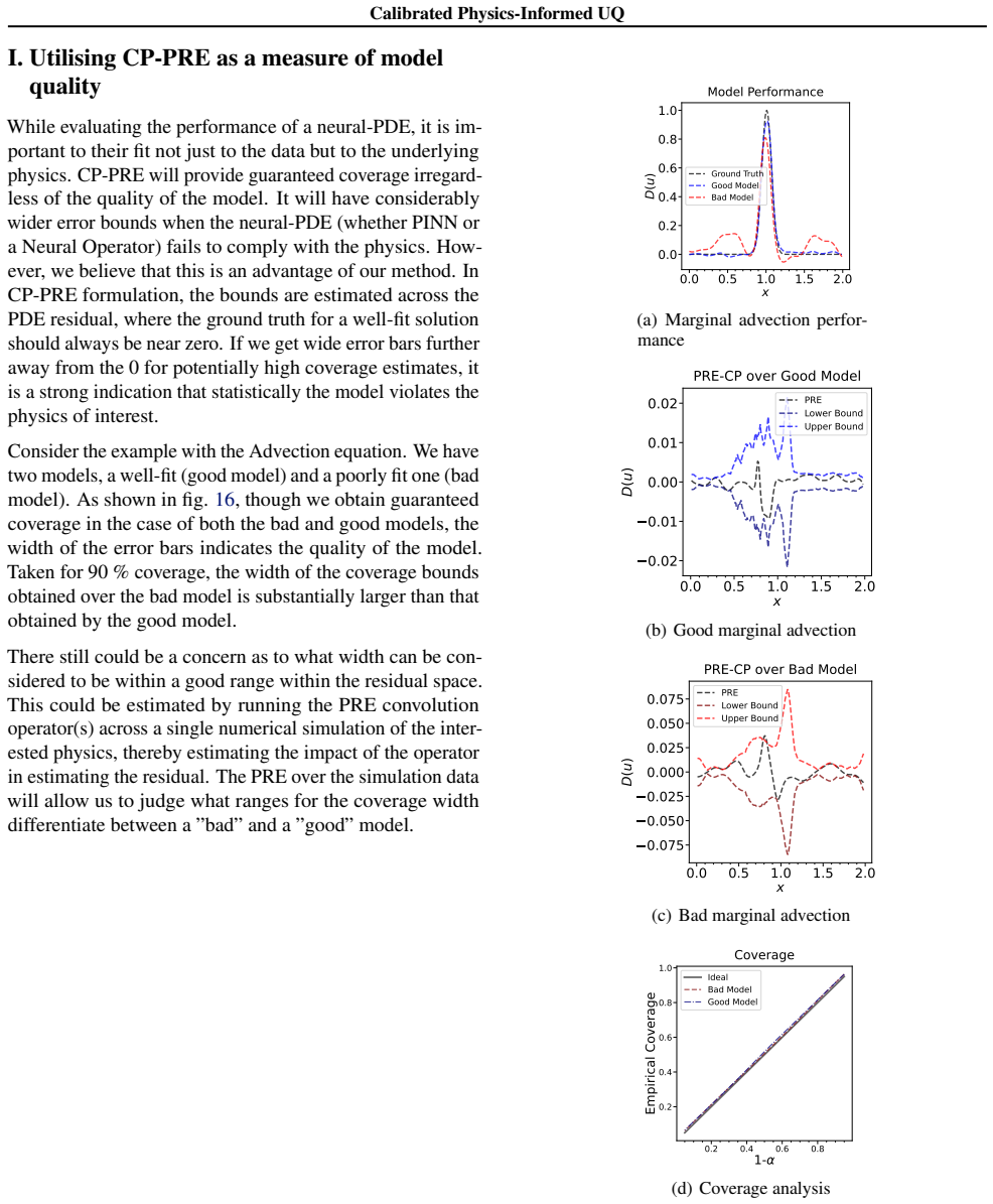
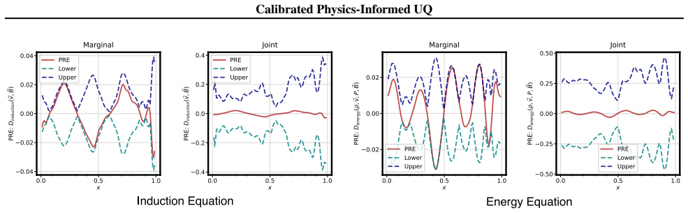
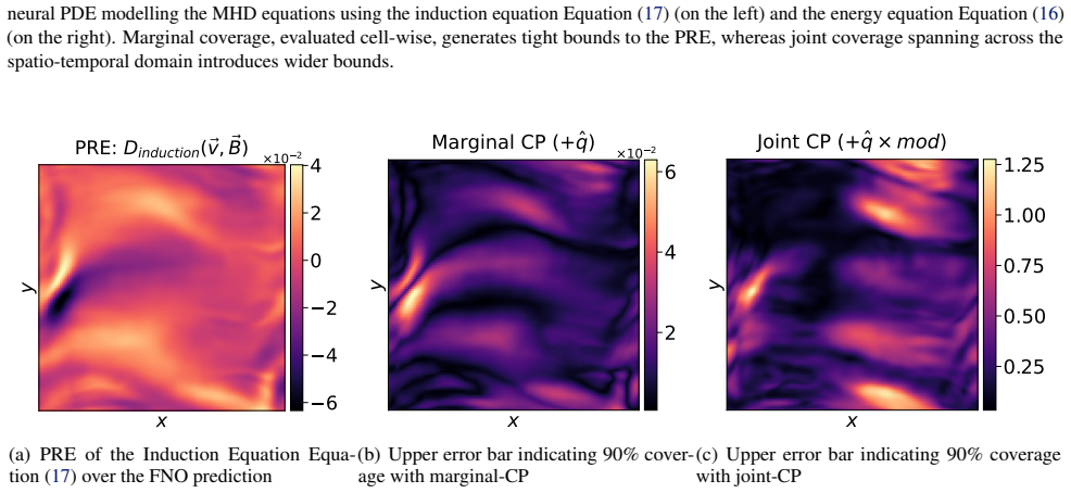
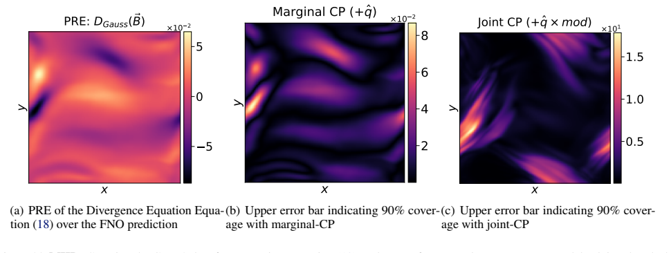
- Marginal CP supplies per-cell error bars that localise spatio-temporal regions where the surrogate violates the physics.
- Joint CP supplies a domain-wide band that can accept or reject whole predictions, enabling a fallback pipeline that routes rejected cases to numerical solvers.
- Guaranteed marginal and joint coverage is reported for wave, Navier-Stokes, magnetohydrodynamic, and two tokamak fusion surrogates (plasma blob evolution and Grad-Shafranov equilibrium).
- The framework extends to any forward model written in the canonical form $Ax - b = 0$, including ODEs and algebraic equations, not just PDEs.
Reading between the lines
- Beyond the paper: the guarantee lives on the residual, so a prediction can satisfy the band and still be wrong in solution space if the added error is annihilated by the differential operator (for example, adding a homogeneous solution of a linear PDE); relying on the band thus assumes the residual is a faithful proxy for solution error.
- Beyond the paper: the theorem's exchangeability assumption means the strong out-of-distribution coverage seen in the experiments should be expected to degrade somewhere; a practical safeguard is to monitor coverage online or re-calibrate on a domain that brackets the deployment distribution.
- Beyond the paper: the joint reject/accept criterion is a natural active-learning signal—retrain the surrogate on the initial conditions whose residuals exceed the band, and the quantile should tighten as the model learns the hard physics cases.
Editorial analysis
A structured set of objections, weighed in public.
Referee Report
Summary. The paper proposes CP-PRE, a conformal prediction framework for neural PDE solvers in which the nonconformity score is the norm of the PDE residual of the surrogate prediction. The framework is post-hoc, model-agnostic, and does not require target labels for calibration: it computes a quantile qhat of calibration residual scores and forms the prediction set [-qhat, qhat] for the residual at a new input. The manuscript presents a theorem claiming marginal coverage under exchangeability, a joint-CP variant, a convolutional finite-difference implementation of residual evaluation, and experiments on the wave, Navier-Stokes, and MHD equations plus two tokamak applications. The paper's headline claims include 'guaranteed coverage across prediction domains' and 'relaxing exchangeability restrictions.'
Significance. If the in-distribution guarantee is correctly stated, CP-PRE is a practically valuable and very cheap UQ scheme for neural PDE surrogates: it turns a physics residual into a calibrated, label-free error bound, and the convolutional stencil implementation is a nice engineering contribution with released code. The in-distribution result follows from standard split conformal prediction applied to a new score, so the core theoretical claim is credible. However, the manuscript substantially overclaims the theoretical scope by presenting out-of-distribution coverage as a derived guarantee and by asserting that the method relaxes exchangeability restrictions; these claims are not consequences of the theorem. The marginal-CP per-cell coverage interpretation also needs clarification, because the validation reports averaged empirical coverage, which is weaker than pointwise per-cell guarantees.
major comments (3)
- [Section 5, Tables 3-5, Theorem A.1] The claim of 'guaranteed coverage for both in and out-of-distribution testing' (Section 5, text above Table 3, and repeated in the abstract as 'coverage guarantees across prediction domains') is not supported by Theorem A.1, which assumes that calibration residuals and the new residual are exchangeable. Under a shifted deployment distribution there is no guarantee that the coverage remains at 1-alpha; the OOD results in Tables 3-5 are empirical observations on unspecified shifts. Moreover, the appendix descriptions for the 1D and 2D experiments state that 'the same bounded domain ... is used for calibration and validation' (Sections G.3, H.3, J.3, K.3, L.2), which makes the nature of the 'out-of-distribution' columns unclear. Please either remove the OOD guarantee language, explicitly describe the actual distribution shift and reframe the results as empirical, or provide a theoretical extension for the specific shift considered.
- [Section 4.1, Figure 3] Section 4.1 states that marginal-CP 'provides independent error bars for each cell' and that the resulting intervals are 'compliant with Equation (5) for each cell.' The implementation appears to compute a single scalar qhat from the pooled cell-wise residuals and then applies this same value to every cell; the empirical validation in Figure 3 reports 'average empirical coverage,' which is consistent with coverage over the pooled distribution rather than per-cell coverage. If the quantile is global, the 'per cell' guarantee is not valid and the language should be revised to state that coverage holds on average over cells. Please clarify the calibration protocol and, if per-cell quantiles are used, specify how they are estimated.
- [Contributions, Section 7] The bullet point in the contributions stating that the method provides 'input-independent prediction sets while relaxing exchangeability restrictions' is incorrect. Theorem A.1 requires exchangeability of the residuals (or of the inputs when the model is fixed); the fact that the prediction set [-qhat, qhat] does not depend on the new input X_{n+1} does not remove or relax this requirement. The related sentence in the Discussion that the framework 'loosens exchangeability restrictions as we can modify the calibration domain by reformulating the PRE' is also unsupported. Please correct these statements to avoid claiming a property that the theory does not provide.
minor comments (5)
- [Appendix A, proof of Theorem A.1] The proof states P(pi(R_{n+1}) <= ceil((n+1)(1-alpha))) = ceil((n+1)(1-alpha))/n. Under exchangeability the rank is uniform on {1, ..., n+1}, so the probability is ceil((n+1)(1-alpha))/(n+1), not over n. The final inequality still holds because ceil((n+1)(1-alpha))/(n+1) >= 1-alpha, but the displayed equality is mathematically incorrect and should be fixed.
- [Section 5.1 and Appendix J] The 'out-of-distribution' columns in Tables 3 and 4 are not accompanied by a definition of the distribution shift. Please state explicitly how the out-of-distribution test initial conditions were sampled (e.g., wider parameter ranges, different PDE coefficients, or a different grid), since the current appendix descriptions suggest that validation uses the same bounded domain as calibration.
- [Table 2] The 'Data-Free' label for CP-PRE could be misleading: the method still requires sampling initial conditions and running the surrogate to generate calibration residuals, although no target labels are needed. Consider using 'Label-Free' or 'Target-Free' to describe the property more precisely.
- [Section B] The sentence 'the true output Y for PRE, irrespective of the PDE is always 0' is confusing because the residual operator D acts on the model output and the score is the norm of that residual field. Please rephrase to clarify that the score measures the deviation from satisfying the PDE, i.e., |D(fhat(X)) - 0|, rather than claiming the output Y itself is zero.
- [Section D.1] Typo: 'control in teh temporal discretisation' should read 'control in the temporal discretisation.' Please proofread throughout.
Circularity Check
The central coverage theorem is a standard split-conformal lemma applied to a new score; the paper's OOD coverage claims exceed the theorem but do not render the derivation circular.
full rationale
Theorem A.1 proves P(|D(f_hat(X_{n+1}))| <= q_hat) >= 1-alpha from exchangeability of the scalar residuals; this is the textbook split-conformal argument and is self-contained in the appendix. The PRE score is a legitimate nonconformity measure: it maps each input to a scalar physics residual, and the calibrated quantile q_hat is not a parameter fitted to the validation targets. The in-distribution coverage experiments are a standard empirical check of this theorem rather than a circular prediction. The abstract and Tables 3-5 additionally claim coverage "across prediction domains" and "out-of-distribution"; these statements are not consequences of Theorem A.1 and would need a separate distribution-shift argument, but an unsupported scope claim is a correctness/validity concern, not a circular reduction. Self-citations to Gopakumar et al. (2024a) are used to justify not re-testing multiple architectures, but the model-agnostic property follows from the CP theorem independently, so no load-bearing argument reduces to the self-citation.
Assumptions & free parameters
free parameters (1)
- residual quantile q_hat =
empirical (ceil((n+1)(1-alpha))/n)-quantile of calibration PRE scores
assumptions (5)
- domain assumption Exchangeability of residuals {|D(f_hat(X_i))|} between calibration and deployment.
- standard math The true solution satisfies the PDE, so its residual is zero.
- domain assumption Finite-difference stencils computed as convolutions approximate the PDE residual up to truncation error.
- domain assumption Boundary conditions are either periodic or disregarded in the main coverage experiments.
- domain assumption The surrogate f_hat is fixed during calibration.
Cite this review
Pith. "Pith review of Calibrated Physics-Informed Uncertainty Quantification." pith.science (2026). https://pith.science/paper/HVBSJF63
@misc{pith2026250204406,
  author       = {Pith},
  title        = {Pith review of: Calibrated Physics-Informed Uncertainty Quantification},
  year         = {2026},
  howpublished = {\url{https://pith.science/paper/HVBSJF63}},
  note         = {Machine review of arXiv:2502.04406}
}
read the original abstract
Simulating complex physical systems is crucial for understanding and predicting phenomena across diverse fields, such as fluid dynamics and heat transfer, as well as plasma physics and structural mechanics. Traditional approaches rely on solving partial differential equations (PDEs) using numerical methods, which are computationally expensive and often prohibitively slow for real-time applications or large-scale simulations. Neural PDEs have emerged as efficient alternatives to these costly numerical solvers, offering significant computational speed-ups. However, their lack of robust uncertainty quantification (UQ) limits deployment in critical applications. We introduce a model-agnostic, physics-informed conformal prediction (CP) framework that provides guaranteed uncertainty estimates without requiring labelled data. By utilising a physics-based approach, we can quantify and calibrate the model's inconsistencies with the physics rather than the uncertainty arising from the data. Our approach utilises convolutional layers as finite-difference stencils and leverages physics residual errors as nonconformity scores, enabling data-free UQ with marginal and joint coverage guarantees across prediction domains for a range of complex PDEs. We further validate the efficacy of our method on neural PDE models for plasma modelling and shot design in fusion reactors.
Figures


Figures from the paper (28 more)








Reference graph
Works this paper leans on
-
[1]
For a new inputX n+1, compute ˆf(X n+1)
-
[2]
17 Calibrated Physics-Informed UQ
Calculate the residual:r=|D( ˆf(X n+1))|. 17 Calibrated Physics-Informed UQ
-
[3]
Check ifr∈[−ˆq α,ˆqα]for a givenα. If the condition in step 3 is satisfied, the error bounds dic- tated by [−ˆqα,ˆqα] is considered valid according to the CP framework, regardless of the specific inputX n+1. C. Algorithmic Procedure 1.Set up the Neural PDE Solver (a) Define the PDE system of interest with its govern- ing equations in a numerical solver (b...
work page 2019
-
[8]
URL https://www.sciencedirect.com/ science/article/pii/S1566253521001081. Actor, J., Fuentes, D. T., and Riviere, B. Identification of kernels in a convolutional neural network: connections between the level set equation and deep learning for im- age segmentation. In Landman, B. A. and Iˇsgum, I. (eds.), Medical Imaging 2020: Image Processing. SPIE, March...
doi:10.1038/150405d0 2020
-
[12]
Li, Z., Zheng, H., Kovachki, N., Jin, D., Chen, H., Liu, B., Azizzadenesheli, K., and Anandkumar, A
URL https://openreview.net/forum? id=c8P9NQVtmnO. Li, Z., Zheng, H., Kovachki, N., Jin, D., Chen, H., Liu, B., Azizzadenesheli, K., and Anandkumar, A. Physics- informed neural operator for learning partial differential equations.ACM / IMS J. Data Sci., 1(3), may 2024. doi: 10.1145/3648506. URL https://doi.org/10. 1145/3648506. Liu, S., Oosterlee, C. W., a...
arXiv 2024
-
[14]
URL https://www.sciencedirect.com/ science/article/pii/S0021999122009652
doi: https://doi.org/10.1016/j.jcp.2022.111902. URL https://www.sciencedirect.com/ science/article/pii/S0021999122009652. Raissi, M., Perdikaris, P., and Karniadakis, G. Physics- informed neural networks: A deep learning frame- work for solving forward and inverse problems involv- ing nonlinear partial differential equations.Journal of Computational Physi...
-
[17]
cc/paper_files/paper/2021/file/ 312f1ba2a72318edaaa995a67835fad5-Paper
URL https://proceedings.neurips. cc/paper_files/paper/2021/file/ 312f1ba2a72318edaaa995a67835fad5-Paper. pdf. Strang, G. A proposal for toeplitz matrix calculations. Studies in Applied Mathematics, 74(2):171–176, 1986. doi: https://doi.org/10.1002/sapm1986742171. URL https://onlinelibrary.wiley.com/doi/ abs/10.1002/sapm1986742171. Sun, S. Conformal method...
arXiv 2021
-
[18]
URL https://proceedings.mlr.press/ v139/xu21h.html. Xu, C., Xie, Y ., Vazquez, D. A. Z., Yao, R., and Qiu, F. Spatio-temporal wildfire prediction using multi-modal data.IEEE Journal on Selected Areas in Information Theory, 4:302–313, 2023. doi: 10.1109/JSAIT.2023. 3276054. Zhu, Y ., Zabaras, N., Koutsourelakis, P.-S., and Perdikaris, P. Physics-constraine...
Show all 24 references
-
[24]
Zou, Z., Meng, X., Psaros, A
URL https://www.sciencedirect.com/ science/article/pii/S0021999119303559. Zou, Z., Meng, X., Psaros, A. F., and Karniadakis, G. E. Neuraluq: A comprehensive library for uncertainty quan- tification in neural differential equations and operators. SIAM Review, 66(1):161–190, 202...
2024
-
[25]
The FNO architecture can be found in Table 13
Each Fourier layer has 8 modes and a width of 16. The FNO architecture can be found in Table 13. We employ a linear range normalisation scheme, placing the field val- ues between -1 and 1. Each model is trained for up to 500 epochs using the Adam optimiser (Kingma & Ba, 2015) ...
2015
-
[45]
URL https://www.sciencedirect.com/ science/article/pii/S0021999118307125. Saad, Y . and Schultz, M. H. Gmres: A generalized mini- mal residual algorithm for solving nonsymmetric linear systems.SIAM Journal on Scientific and Statistical Com- puting, 7(3):856–869, 1986. doi: 10....
1986 doi
-
[565]
URL https: //doi.org/10.1023/A:1020281327116
doi: 10.1023/A:1020281327116. URL https: //doi.org/10.1023/A:1020281327116. Angelopoulos, A. N. and Bates, S. Conformal prediction: A gentle introduction.Found. Trends Mach. Learn., 16 (4):494–591, mar 2023. ISSN 1935-8237. doi: 10.1561/ 2200000101. URL https://doi.org/10.1561...
2023
-
[2012]
doi: 10.1007/ 978-1-4614-4283-7 19
ISBN 978-1-4614-4283-7. doi: 10.1007/ 978-1-4614-4283-7 19. URL https://doi.org/ 10.1007/978-1-4614-4283-7_19. Stankeviciute, K., M. Alaa, A., and van der Schaar, M. Con- formal time-series forecasting. In Ranzato, M., Beygelz- imer, A., Dauphin, Y ., Liang, P., and Vaughan, J...
-
[2014]
Li, Z., Kovachki, N
doi: 10.1155/2014/940965. Li, Z., Kovachki, N. B., Azizzadenesheli, K., liu, B., Bhat- tacharya, K., Stuart, A., and Anandkumar, A. Fourier neu- ral operator for parametric partial differential equations. InInternational Conference on Learning Representations,
2014 doi
-
[2015]
The learning rate is initially set to 0.005 and scheduled to decrease by half after every 100 epochs
with a step-decaying learning rate. The learning rate is initially set to 0.005 and scheduled to decrease by half after every 100 epochs. The model was trained using an LP-loss (Gopakumar et al., 2024b). Table 9. Architecture of the 1D FNO deployed for modelling 1D Burgers’ eq...
-
[2019]
cc/paper_files/paper/2019/file/ 118921efba23fc329e6560b27861f0c2-Paper
URL https://proceedings.neurips. cc/paper_files/paper/2019/file/ 118921efba23fc329e6560b27861f0c2-Paper. pdf. McCabe, M., Harrington, P., Subramanian, S., and Brown, J. Towards stability of autoregressive neural opera- tors.Transactions on Machine Learning Research, 2023. ISSN...
2019
-
[2020]
cc/paper_files/paper/2020/file/ d16a974d4d6d0d71b29bfbfe045f1da7-Paper
URL https://proceedings.neurips. cc/paper_files/paper/2020/file/ d16a974d4d6d0d71b29bfbfe045f1da7-Paper. pdf. Eymard, R., Gallou ¨et, T., and Herbin, R. Finite volume methods. In Lions, J. L. and Ciarlet, P. (eds.),Solution of Equation in Rn (Part 3), Techniques of Scientific ...
2020 doi
-
[2021]
URL https: //dx.doi.org/10.1088/1741-4326/abf99f
doi: 10.1088/1741-4326/abf99f. URL https: //dx.doi.org/10.1088/1741-4326/abf99f. Horwitz, J. A. K. Estimating the carbon footprint of compu- tational fluid dynamics.Physics of Fluids, 36(4):045109, 04 2024. ISSN 1070-6631. doi: 10.1063/5.0199350. URLhttps://doi.org/10.1063/5.0...
2024 arXiv
-
[2023]
Kingma, D
URL https://proceedings.mlr.press/ v204/kato23a.html. Kingma, D. P. and Ba, J. Adam: A method for stochas- tic optimization. In Bengio, Y . and LeCun, Y . (eds.), 3rd International Conference on Learning Represen- tations, ICLR 2015, San Diego, CA, USA, May 7-9, 2015, Conferen...
2015 arXiv
-
[2322]
URL https: //doi.org/10.1038/s41598-023-42991-5
doi: 10.1038/s41598-023-42991-5. URL https: //doi.org/10.1038/s41598-023-42991-5. Karniadakis, G. E., Kevrekidis, I. G., Lu, L., Perdikaris, P., Wang, S., and Yang, L. Physics-informed ma- chine learning.Nature Reviews Physics, 3(6):422– 440, 2021. ISSN 2522-5820. doi: 10.1038...
-
[4435]
URL https: //doi.org/10.1038/s43247-024-01885-8
doi: 10.1038/s43247-024-01885-8. URL https: //doi.org/10.1038/s43247-024-01885-8. Giudicelli, G., Lindsay, A., Harbour, L., Icenhour, C., Li, M., Hansel, J. E., German, P., Behne, P., Marin, O., Stogner, R. H., Miller, J. M., Schwen, D., Wang, Y ., Munday, L., Schunert, S., Sp...
-
[4687]
URL https: //doi.org/10.1038/s41586-024-07744-y
doi: 10.1038/s41586-024-07744-y. URL https: //doi.org/10.1038/s41586-024-07744-y. Lakshminarayanan, B., Pritzel, A., and Blundell, C. Simple and scalable predictive uncertainty estimation using deep ensembles, 2017. Lao, L., St. John, H., Stambaugh, R., Kellman, A., and Pfeiff...
2017 doi
-
[7110]
URL https://www.sciencedirect.com/ science/article/pii/S235271102400061X
doi: https://doi.org/10.1016/j.softx.2024.101690. URL https://www.sciencedirect.com/ science/article/pii/S235271102400061X. Gopakumar, V . and Samaddar, D. Image mapping the tem- poral evolution of edge characteristics in tokamaks using neural networks.Machine Learning: Scienc...
2024
-
[9991]
URL https://www.sciencedirect.com/ science/article/pii/S0021999119307612
doi: https://doi.org/10.1016/j.jcp.2019.109056. URL https://www.sciencedirect.com/ science/article/pii/S0021999119307612. Giles, D., Briant, J., Morcrette, C. J., and Guillas, S. Em- bedding machine-learnt sub-grid variability improves climate model precipitation patterns.Comm...
2019
Reviewed August 9, 2026 · model on record in the stance chip above.
Discussion (0). Continue with ORCID to comment.