REVIEW 6 major objections 6 minor 1 cited by
Data-driven Approach for Interpolation of Sparse Data
T0 review · 6 major / 6 minor · reviewed 2026-08-16 · deepseek-v4-flash
Pith's one-line read Gaussian processes can interpolate sparse hadron data with quantified uncertainties, removing the need for arbitrary weighting.
desk verdict A useful applied-GP recipe for sparse hadron data, but the calibration evidence is circular and the headline robustness claim outruns the validation. read the letter →
The pith
A machine-rendered reading of the paper's core claim, the machinery that carries it, and where it could break.
The reading
What carries the argument
The engine is a Gaussian process with an RBF kernel $\kappa(\vec a,\vec b,\vec l)=\exp(-\sum_k \|a_k-b_k\|^2/(2 l_k^2))$, whose prediction for an unmeasured point is the conditional mean $\vec\mu_* = K_*^T K^{-1}\vec y$ and covariance $\Sigma_* = K_{**}-K_*^T K^{-1} K_*$. Because the log marginal likelihood of Eq. (1) is unstable for sparse data, the authors introduce the coverage-loss function $f(\vec l)=\int_0^3 |M(c\sigma,\vec l)-P(c\sigma)|\,dc$ of Eq. (2), which scores how well the GP's error bands contain the expected fraction of points. The loss is minimised with a standard minimiser in 1D and, in higher dimensions, by MCMC sampling followed by K-means clustering with silhouette scoring to pick among the loss surface's multiple modes; predictions are restricted to the convex hull of the measured points, with bin edges added when binning information is available.
What would settle it
Take a sparse pseudodataset with a known generating function, compute the coverage-loss-optimal length scale and the marginal-likelihood-optimal length scale, and compare predictive mean squared error and empirical coverage on out-of-sample points; if the coverage-loss choice is no better than the marginal likelihood and its uncertainty bands undercover on held-out points, the central claim fails. The paper's Table I already measures in-sample pull, so a fully independent check requires points not used in the GP fit.
Extended reading notes
Core claim
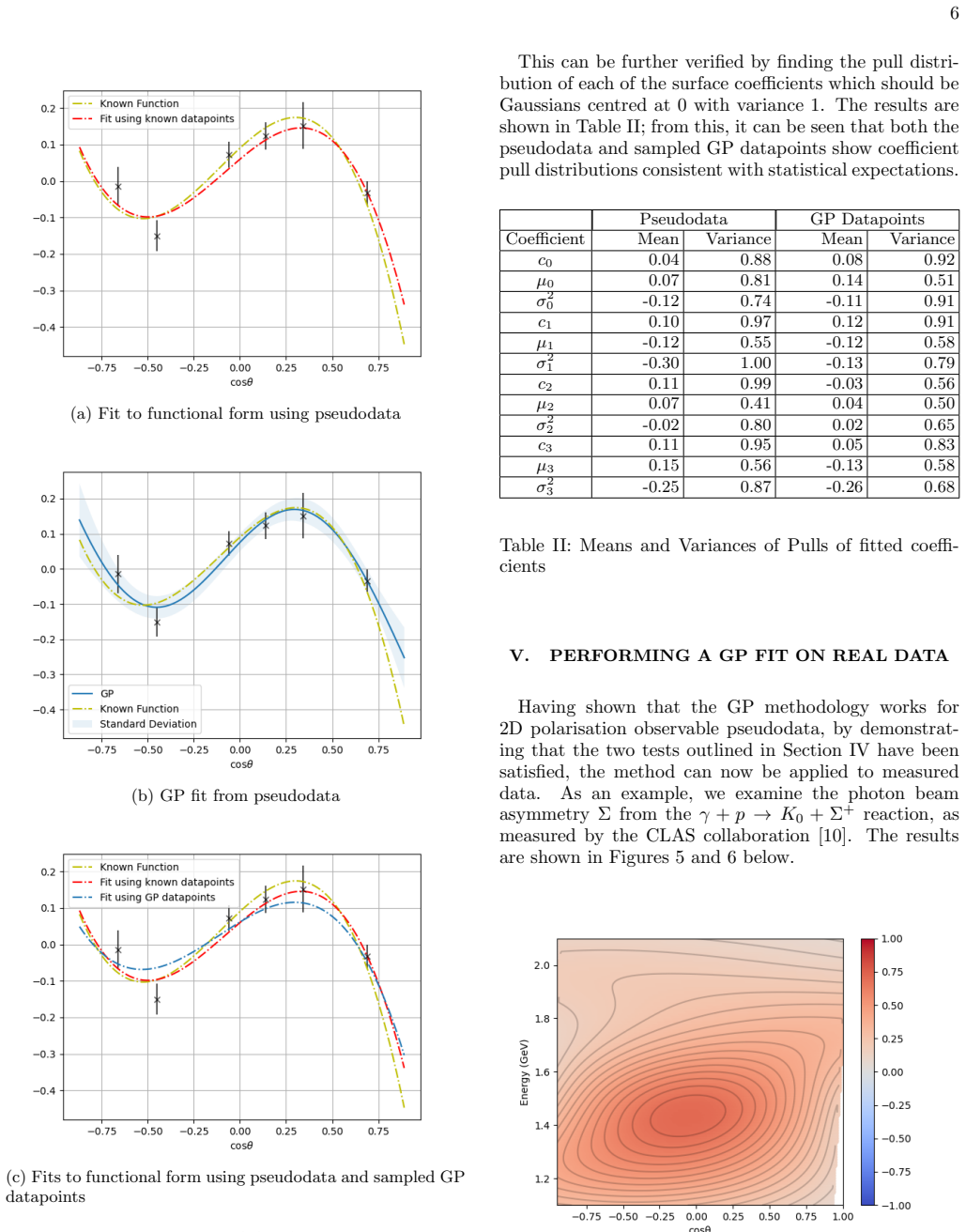
The central claim is that a Gaussian process whose radial-basis-function length scales are optimised against a coverage loss—the integrated absolute difference between the observed and expected fractions of training points inside $0$ to $3\sigma$ bands of the GP mean—interpolates sparse hadron-spectroscopy datasets as accurately as the original data themselves, with well-quantified uncertainties. The paper demonstrates this by showing that pull distributions of sampled GP points match statistical expectations and that fits to the known functional form using GP-sampled points reproduce fits to the original pseudodata. It further claims the same machinery can expose inconsistencies between experiments, as illustrated by a double-ridged log-probability surface for $K^-p\to \bar{K}^0 n$ world data, where a least-squares fit would sit between the ridges and miss the maximum likelihood.
Load-bearing premise
The load-bearing premise is that the coverage-based loss computed on the training data is a valid replacement for the marginal likelihood in choosing length scales, and that in-sample coverage checks plus GP-sampled points are enough to certify the interpolated values and uncertainties.
Editorial extensions
If this is right
- Fits of coupled-channels models can use GP-interpolated points with the same kinematic density for every observable, removing experiment-specific relative weights.
- A combined probability surface built from individual GP fits can replace a single weighted average when datasets disagree, preventing least-squares fits from landing in low-probability valleys.
- The method supplies a value and uncertainty at any kinematic point inside the measured domain, enabling model tests in kinematic regions where no direct measurement exists.
- The same GP treatment can be applied to any observable of a reaction, so all measured quantities enter a theoretical fit in the same way.
Reading between the lines
- The coverage loss is a frequentist calibration criterion rather than a proper scoring rule; for very small samples the step-like 1$\sigma$ curve in Fig. 1 suggests the minimum may be sensitive to the discrete placement of points, so a bootstrap or repeated-pseudodata study of length-scale stability would be a natural extension.
- Because the GP uncertainty is itself an estimate, any downstream fit that treats GP-sampled points as independent data will understate the total uncertainty; a two-stage analysis should propagate the GP covariance or use the full posterior predictive distribution.
- The consistency-surface idea could be turned into a quantitative disagreement measure, such as overlap integrals between experiment-specific GP posteriors, and applied to other multi-experiment fields like lattice QCD averages or nuclear reaction databases.
- If the coverage loss were replaced by a proper scoring rule evaluated on a small validation set, the method might combine the stability of the coverage criterion with the statistical guarantees of the marginal likelihood.
Signed reviews
Editorial analysis
A structured set of objections, weighed in public.
Referee Report
Summary. This paper proposes a Gaussian-process (GP) interpolation method intended to replace arbitrary weighting of sparse hadron spectroscopy data. The proposed model uses a squared-exponential (RBF) kernel, and the length-scale hyperparameters are selected by minimizing a coverage-loss function f(l) defined in Eq. (2), which compares the empirical fraction of training points inside c-sigma bands with the Gaussian expectation; the minimization is performed with MCMC and K-means clustering. The authors validate the method on 100 pseudodata surfaces made of Legendre polynomials times Gaussian energy functions (Eq. (4)), then apply it to CLAS photon-beam asymmetry data and to seven experiments for K-p -> Kbar0 n, constructing a combined probability surface to assess dataset consistency.
Significance. If the validation were trustworthy, the method would be a convenient and transferable recipe for hadron spectroscopy analyses, and the manuscript is generally clear and backed by a public code repository. However, the evidence as presented does not support the central robustness claim: the hyperparameter-selection criterion and the headline calibration statistic are the same quantity, the 'GP datapoints' are not an independent test, the pseudodata are unrealistically smooth, and the MCMC procedure is not Bayesian in any standard sense. With an independent held-out validation and a defensible hyperparameter-selection scheme, the tool could be of practical value to the hadron-spectroscopy community.
major comments (6)
- [III B and Table I] The coverage-loss function f(l) in Eq. (2) and the validation statistic in Table I are the same object. The 'Known Points' column reports M(csigma,l) after l is chosen to minimize |M(csigma,l)-P(csigma)|, so the displayed agreement is enforced by construction. The in-sample coverage numbers therefore do not constitute evidence of calibrated GP uncertainties; a held-out validation set or a cross-validation scheme is required.
- [III B, Appendix B] The manuscript repeatedly calls the procedure 'Bayesian inference' (Abstract, Section III B), but f(l) is an ad hoc loss, not a likelihood or posterior, so running MCMC on it does not yield posterior samples or hyperparameter uncertainties. In addition, Appendix B sets T_w=0 for the integrated autocorrelation time, which makes tau_w=1/2 and tau_stability=0 for every chain; the stated autocorrelation convergence criterion is thus vacuous. The convergence assessment therefore rests only on the Gelman-Rubin statistic, and the claim of Bayesian hyperparameter optimization is unsupported.
- [IV A and Table I] The 'GP Points' column does not validate interpolation at unobserved kinematics. These points are drawn from the GP predictive distribution conditioned on the same training data, so they are not independent of the hyperparameter choice and cannot reveal miscalibration away from the training points. The text's assertion that the GP can use the full dataset 'without arbitrary splitting' does not remove the need for an external validation; leave-one-energy-out or a separate test surface would be a minimal fix.
- [Table II] Table II does not support the stated conclusion. For the GP datapoints the pull variances include mu0=0.51, c2=0.56, mu2=0.50, and sigma2_3=0.68; even the pseudodata column has mu2=0.41 and mu1=0.55. Since a correctly calibrated pull distribution has variance 1, these values indicate overestimated fit uncertainties or neglected correlations. The claim that both columns are 'consistent with statistical expectations' is contradicted by the reported numbers.
- [IV, Eq. (4)] The validation family in Eq. (4) consists of four low-order Legendre polynomials times Gaussian energy functions, which are smooth and broad. Typical hadron resonance datasets contain narrow peaks, threshold effects, and rapid angular structure; the abstract's claim that GPs are robust for 'typical datasets used in hadron resonance studies' is not established by tests on this unrealistically smooth family. Adding sharp-featured test functions is essential to support the generality claim.
- [VI] The combined probability surface is not a proper likelihood. Summing normalized Gaussian GP predictive densities from independent experiments and renormalizing at each energy treats the experiments as independent likelihood terms with no common-systematic component and ignores correlations within each GP fit. The plot in Figure 8 may be a useful heuristic diagnostic, but the claim that a least-squares fit would produce 'misleading inferences' because it is not maximum likelihood requires this surface to be a valid likelihood, which is not shown.
minor comments (6)
- [Eq. (2)] The notation '3X c>0' for the discrete approximation of the integral is non-standard; the sum over a grid of c values in (0,3] should be written explicitly.
- [III B] The phrase 'predicated percentage' should be 'predicted percentage'.
- [II] The covariance matrix is defined inconsistently: first as K = kappa(X,X) + vector e^2 I_n and then correctly as K_ab = kappa(x_a,x_b) + delta_ab e_a^2; the vector notation should be removed or defined.
- [Table I] The measured percentages are quoted without statistical uncertainties; with 100 pseudodata surfaces and variable numbers of points, the sampling error on each percentage should be reported.
- [III C] The angle-bin-width formula uses symbols m and a_m without definition; the indexing for degenerate datapoints should be stated explicitly.
- [Reference [3]] The GitHub repository is cited without a version or commit identifier; for reproducibility, please include the commit hash or an archived DOI.
Circularity Check
In-sample coverage validation restates the fitted loss; remaining pseudodata checks are only partly independent, so partial circularity.
-
self definitional
[Section III B (Eq. 2) and Section IV A (Table I)]
"f(⃗l) = ∫_0^3 |M(cσ,⃗l)−P(cσ)|dc ≈ Σ_{c>0} |M(cσ,⃗l)−P(cσ)|, (2) ... M(cσ,⃗l) is the measured percentage of datapoints falling within cσ of the GP mean for a given length scale ⃗l ... Table I: Different σ bands and the measured percentage of points contained in each ... Measured Percentage of Known Points (%) 51.2 68.1 94.8"
The length scale is selected by minimizing f(⃗l), which is literally the integrated absolute difference between the measured coverage M(cσ,⃗l) of the known training points and the nominal Gaussian coverage P(cσ). Table I's 'Known Points' column reports exactly this same M(cσ,⃗l) at the selected length scale (51.2%, 68.1%, 94.8% against the expected 50%, 68.3%, 95%). The in-sample agreement is therefore imposed by the selection objective: it restates the fitted target rather than independently confirming that the GP predictive variances are calibrated. The 'GP Points' column is a separate check, but it is conditional on the length scale already chosen from the training coverage and on smooth pseudodata generated from Eq.
full rationale
The central methodological novelty is Eq. (2), a coverage-deficit loss used to choose GP length scales and to support the claim of robust, quantified uncertainties. The validation in Table I has a 'Known Points' column that is the same statistic the loss minimizes, making that part of the validation self-definitional. The 'GP Points' column and the coefficient-pull tests in Section IV B provide some independent evidence that interpolation on smooth Legendre-Gaussian pseudodata preserves the underlying functional form, and the real-data applications are demonstrations rather than tests of the method. There is no load-bearing self-citation chain: the citations to Rasmussen and Williams and to standard MCMC packages are external support. However, because the headline robustness and uncertainty-quantification claim rests in part on the circular known-points coverage check, and because the ad hoc loss is introduced without derivation from a likelihood, the paper is partially circular rather than fully self-contained.
Assumptions & free parameters
free parameters (3)
- RBF length scale l_k (per kinematic dimension) =
not reported; selected by minimizing Eq. (2)
- Integration range c in (0,3] =
c_max = 3
- MCMC convergence thresholds =
Rhat < 1.18; tau_stability < 0.15
assumptions (6)
- domain assumption The RBF kernel is a valid covariance model for the hadron observables being interpolated.
- ad hoc to paper The fraction of data points within c sigma of the GP mean should match the Gaussian expected fraction, and minimizing this mismatch is a valid hyperparameter selection rule.
- ad hoc to paper A GP can be validated using the same data used for hyperparameter optimization, without a held-out split.
- ad hoc to paper The sum of normalized Gaussian predictions from different experiments is a valid combined probability surface.
- domain assumption The quoted measurement uncertainties are independent, Gaussian, and accurate.
- standard math Standard Gaussian process and multivariate Gaussian conditioning results are valid.
Cite this review
Pith. "Pith review of Data-driven Approach for Interpolation of Sparse Data." pith.science (2026). https://pith.science/paper/6JAJYK2F
@misc{pith2026250501473,
  author       = {Pith},
  title        = {Pith review of: Data-driven Approach for Interpolation of Sparse Data},
  year         = {2026},
  howpublished = {\url{https://pith.science/paper/6JAJYK2F}},
  note         = {Machine review of arXiv:2505.01473}
}
read the original abstract
Studies of hadron resonances and their properties are limited by the accuracy and consistency of measured datasets, which can originate from many different experiments. We have used Gaussian Processes (GP) to build interpolated datasets, including quantification of uncertainties, so that data from different sources can be used in model fitting without the need for arbitrary weighting. GPs predict values and uncertainties of observables at any kinematic point. Bayesian inference is used to optimise the hyperparameters of the GP model. We demonstrate that the GP successfully interpolates data with quantified uncertainties by comparison with generated pseudodata. We also show that this methodology can be used to investigate the consistency of data from different sources. GPs provide a robust, model-independent method for interpolating typical datasets used in hadron resonance studies, removing the limitations of arbitrary weighting in sparse datasets.
Figures


Figures from the paper (4 more)


Forward citations
Cited by 1 Pith paper
-
Universal parameters of the $\Lambda(1380)$, the $\Lambda(1405)$ and their isospin partners from a combined analysis of Lattice QCD and experimental results
A combined global fit of lattice QCD spectra and experimental Kbar N data within chiral unitary approaches gives pole positions for the Lambda(1380) and Lambda(1405) at physical and lattice quark masses, with systemat...
Reference graph
Works this paper leans on
-
[1]
Some kernel function can be defined to measure the covariance between known datapoints
-
[2]
This same kernel function can be used to predict the covariance between unknown datapoints
-
[3]
Some idea of the form of the posterior distribution is known (e.g. smoothness, continuity, periodicity). This framework enables GPs to interpolate datasets and provide predicted values and uncertainties, which ensures that the quantification of uncertainties is well-defined. Furthermore, the full dataset can be utilised without the need for arbitrary spli...
arXiv 2025
-
[4]
C. E. Rasmussen and C. K. I. Williams, Gaussian Pro- cesses for Machine Learning (MIT Press, 2006) chapter 5: Model Selection and Adaptation of Hyperparameters. 10
work page 2006
-
[5]
K. P. Murphy, Machine Learning: A Probabilistic Per- spective (MIT Press, Cambridge, MA, 2012)
work page 2012
-
[6]
Ferguson, Gaussian-process, https://github.com/ rferguson22/Gaussian-Process, accessed: 2025-05-01
R. Ferguson, Gaussian-process, https://github.com/ rferguson22/Gaussian-Process, accessed: 2025-05-01
work page 2025
-
[7]
F. Pedregosa et al., Scikit-learn: Machine learning in Py- thon, Journal of Machine Learning Research 12, 2825 (2011)
work page 2011
- [8]
Show all 21 references
-
[9]
Foreman-Mackey, D
D. Foreman-Mackey, D. W. Hogg, D. Lang, and J. Good- man, emcee: The MCMC Hammer, Publications of the Astronomical Society of the Pacific 125, 306 (2013), arXiv:1202.3665 [astro-ph.IM]
2013 arXiv
-
[10]
P. J. Rousseeuw, Silhouettes: A graphical aid to the in- terpretation and validation of cluster analysis, Journal of Computational and Applied Mathematics 20, 53 (1987)
1987
-
[11]
Virtanen et al
P. Virtanen et al. , SciPy 1.0: Fundamental Algorithms for Scientific Computing in Python, Nature Methods 17, 261 (2020)
2020
-
[12]
Forcey, G
S. Forcey, G. Hamerlinck, L. Keefe, and W. Sands, The minimum evolution problem in phylogenetics: Polytopes, linear programming, and interpretation, in MSE/Mathematics in Science and Engineering, Algeb- raic and Combinatorial Computational Biology (Aca- demic Press, 2019) Chap. 10
2019
-
[13]
Clark et al
L. Clark et al. (The CLAS Collaboration), Photoproduc- tion of the Σ + hyperon using linearly polarized photons with CLAS, Phys. Rev. C 111, 025204 (2025)
2025
-
[14]
Dembinski, H
H. Dembinski, H. Schreiner, L. Heinrich, and E. Rodrig- ues, iminuit - A Python interface to Minuit, the robust function minimiser, arXiv preprint (2023), arXiv:2301.13072 [physics.comp-ph]
2023 arXiv
-
[15]
Ciborowski et al
J. Ciborowski et al. , Kaon scattering and charged sigma hyperon production in K −p interactions below 300 MeV/c, Journal of Physics G: Nuclear Physics 8, 13 (1982)
1982
-
[16]
Kittel, G
W. Kittel, G. Otter, and I. Wacek, The k- proton charge exchange interactions at low energies and scattering lengths determination, Physics Letters 21, 349 (1966)
1966
-
[17]
J. K. Kim, Multichannel phase-shift analysis of Kn in- teraction in the region 0 to 550 MeV/c, Phys. Rev. Lett. 19, 1074 (1967)
1967
-
[18]
W. E. Humphrey and R. R. Ross, Low-energy interac- tions of K − mesons in hydrogen, Phys. Rev. 127, 1305 (1962)
1962
-
[19]
T. S. Mast et al. , Elastic, charge-exchange, and total K −p cross sections in the momentum range 220 to 470 MeV/c, Phys. Rev. D 14, 13 (1976)
1976
-
[20]
G. S. Abrams and B. Sechi-Zorn, Charge-exchange scat- tering of low-energyK − mesons in hydrogen, Phys. Rev. 139, B454 (1965)
1965
-
[21]
Evans et al
D. Evans et al. , Charge-exchange scattering in K −p in- teractions below 300 MeV/c, Journal of Physics G: Nuc- lear Physics 9, 885 (1983)
1983
Reviewed August 16, 2026 · model on record in the stance chip above.
Discussion (0). Continue with ORCID to comment.