Improved Uncertainty Quantification in Physics-Informed Neural Networks Using Error Bounds and Solution Bundles

Karim Pichara; Olga Graf; Pablo Flores; Pavlos Protopapas

REVIEW 5 major objections 5 minor 12 references

Improved Uncertainty Quantification in Physics-Informed Neural Networks Using Error Bounds and Solution Bundles

T0 review · 5 major / 5 minor · reviewed 2026-08-15 · deepseek-v4-flash

Challenge this review Re-run · record.json Download PDF Read on arXiv ↗ Review JSON

Pith's one-line read The paper's central assertion is that using residual-based error bounds to define a heteroscedastic likelihood variance in a two-step Bayesian training scheme substantially improves calibration of physics-informed neural network…

desk verdict A promising but unproven heuristic: setting the likelihood variance equal to a deterministic PINN error bound can improve calibration, yet the paper never validates that the bound behaves like a Gaussian noise scale. read the letter →

arxiv 2505.06459 v2 pith:HEH7TLLZ submitted 2025-05-09 cs.LG cs.AIphysics.comp-phstat.ML

Pablo Flores , Olga Graf , Pavlos Protopapas , Karim Pichara This is my paper · ORCID

classification cs.LGcs.AIphysics.comp-phstat.ML

keywords physics-informedneuralnetworksuncertaintyquantificationBayesianerrorboundssolutionbundlesheteroscedasticitycosmologicalmodelsinverseproblems

verification ladder T0 review T1 audit T2 compute T3 formal

The pith

A machine-rendered reading of the paper's core claim, the machinery that carries it, and where it could break.

The reading

This paper claims that uncertainty estimates for physics-informed neural networks become substantially better calibrated if the noise scale of the Bayesian likelihood is tied to a worst-case residual error bound rather than a constant. The proposed two-step procedure first trains a deterministic Solution Bundle, a network that takes equation parameters as extra inputs, and then trains a Bayesian network on that deterministic solution, setting the likelihood standard deviation $\sigma_{\mathrm{Like}}(x,\lambda)$ equal to the error bound $B(x,\lambda)$. On four cosmological differential-equation models, the method reduces miscalibration area relative to residual-likelihood baselines and produces parameter posteriors for inverse problems that largely agree with literature values. The sympathetic reading is that this gives practitioners calibrated predictive distributions for PINN solutions without external data.

What carries the argument

The load-bearing object is the error bound $B(x,\lambda)$: a deterministic scalar function computed from the differential equation's coefficients and the PINN's residual, satisfying $\|\eta(x,\lambda)\nleq B(x,\lambda)$ for the approximation error $\eta$. The paper's pivotal move is the substitution $\sigma_{\mathrm{Like}}(x,\lambda)=B(x,\lambda)$, turning a worst-case deterministic bound into the standard deviation of a Gaussian likelihood in the Bayesian second step. The second carrier is the Solution Bundle, a network $u_\theta(x,\lambda)$ trained over a range of equation parameters $\lambda$ in one pass, which supplies the target outputs for the Bayesian network and makes inverse problems tractable because no retraining per parameter is needed.

What would settle it

Compute the empirical distribution of the deterministic error $\eta(x,\lambda)=u_{\mathrm{true}}-\tilde{u}_{\theta_{\mathrm{det}}}$ across a dense grid for the ΛCDM and CPL models, and compare it with $\mathcal{N}(0,B(x,\lambda)^2)$. If the true coverage of the reported 68% and 95% predictive intervals deviates substantially from nominal levels, or if replacing $B$ by a fraction $cB$ with $c<1$ does not change the miscalibration area, the central identification of the error bound as a likelihood variance is not doing the claimed work.

Watch

Extended reading notes

Core claim

The paper's central discovery is the identification of the error bound as a heteroscedastic variance for Bayesian inference: $\sigma_{\mathrm{Like}}(x,\lambda)=B(x,\lambda)$, where $B$ is a deterministic, residual-based upper bound on the solution error. In the two-step scheme, the first step trains a deterministic Solution Bundle by minimizing residuals; the second step uses its outputs as noise-free targets for a Bayesian neural network whose likelihood variance is either constant or equal to $B$. The paper argues that the error-bound choice consistently lowers miscalibration area compared with residual-likelihood baselines and with a homoscedastic variance, while also enabling inverse-problem parameter estimation through marginalization over the predictive distribution. The authors present the result as a trade-off: accuracy is sacrificed relative to the deterministic network, but the calibrated uncertainty is the intended product.

Load-bearing premise

The load-bearing premise is that the worst-case deterministic error bound $B(x,\lambda)$ can be treated as the standard deviation of a Gaussian likelihood; if the actual errors are not Gaussian with that scale, the reported calibration improvement is an artifact of intervals that are forced wide enough to cover the deterministic error by construction.

Editorial extensions

If this is right

If the central claim is right, PINN practitioners can obtain calibrated predictive intervals for forward solutions of ODE systems using only residuals and equation structure, with no external solution data.
The same predictive distributions can be fed into a Bayesian parameter-estimation loop, giving posterior means and error bars for cosmological parameters such as $\Omega_{m,0}$ and $H_0$.
The error-bound variance is architecture-independent, so the calibration benefit should transfer to any Bayesian network used in the second step, including neural linear models, Bayes-by-backpropagation, and Hamiltonian Monte Carlo.
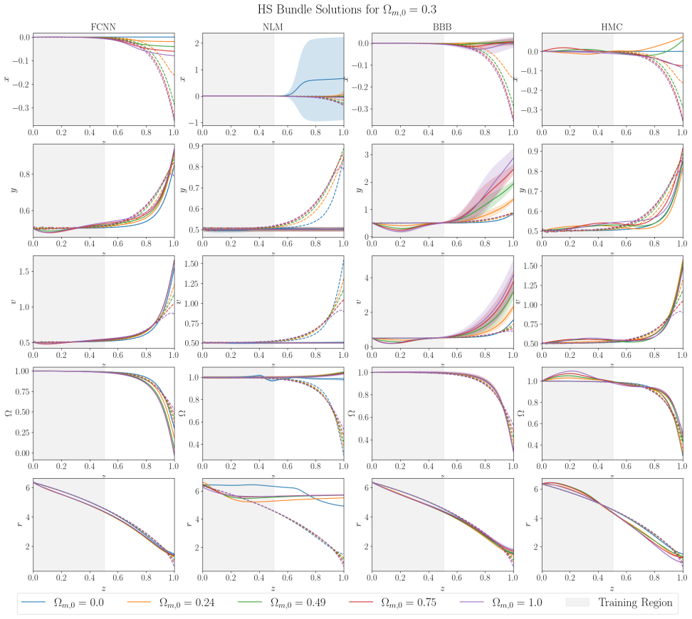
Calibration gains concentrate in the training region; out-of-distribution behavior is mixed, so the method is a statement about in-distribution uncertainty quantification rather than extrapolation.
A trade-off appears: intervals become wider and numerically noisier, particularly for the more complex cosmological models, so calibration at the cost of sharpness is a deliberate choice.

Reading between the lines

Editorial extensions of the paper, not claims the author makes directly.

I would expect the calibration improvement to be partly a consequence of the bound's conservativeness: $B$ is a worst-case upper bound, so intervals must cover the deterministic error by construction; a natural test is to compare against a heteroscedastic variance estimated from empirical error quantiles, which should give similar coverage with narrower intervals if the error distribution is well
The method implicitly assumes the deterministic error is approximately Gaussian at scale $B$; the paper's own histograms show some models are noticeably non-Gaussian, so applying the same recipe to strongly non-Gaussian error distributions would require a different likelihood family.
Because $B$ is available for certain linear and weakly nonlinear ODEs, the technique should transfer to other areas where residual-based PINN bounds exist, such as linear PDEs, provided the bound is evaluated on the parameter-augmented domain.

Share X Bluesky LinkedIn Reddit HN

Signed reviews

No signed human review yet.

Editorial analysis

A structured set of objections, weighed in public.

Desk editor's note, referee report, and a circularity audit.

Desk Editor's Note

read the letter

Pablo and colleagues propose training a deterministic PINN solution bundle, then training a BNN on its outputs with the likelihood standard deviation set to a residual-based error bound B(x,λ). That specific construction is new as far as I know, and the cosmological testbed (ΛCDM, CPL, Quintessence, HS) is a reasonable place to see whether it works. Credit where due: they ship code, they report a range of uncertainty metrics, and they are frank about OOD failures and numerical blow-ups in CPL/HS. The two-step recipe itself is a useful engineering pattern.

The load-bearing step is where I get off the train. Setting σ_Like = B treats a worst-case deterministic error bound as a Gaussian noise scale. A bound is not a standard deviation; a Gaussian with σ=B gives 68% coverage at one sigma, while a bound implies 100%. The paper never checks the empirical distribution of η = u − u_θ_det. Appendix I looks at the distribution of solutions during training, not at the error process. There is also an object mismatch: B bounds u − u_θ_det, but the likelihood is centered on the BNN output u_θ and fitted to u_θ_det. That transfer works only if the BNN posterior mean is close to u_θ_det everywhere. Table 2 already shows a median RE of 0.047 for BBB+2S+EB on ΛCDM, and the OOD tables show the posterior mean drifting well outside the bound's regime. So the reported calibration gains are not as cleanly attributable to 'using the error bound' as the paper claims.

Other soft spots: the 'testing region' in Table 2 is never defined; the training/OOD split in Tables 3–4 is clearer but paints a mixed picture, with some catastrophic CPL/HS results. All metrics appear to come from a single run, with no error bars or sensitivity analysis over σ_Like, σ_prior, or the partition parameters N and K.

I don't think the idea is dead. The heuristic may well be useful: error bounds are cheap to compute and encode where the deterministic net is bad, so using them to inflate predictive variance in those regions is plausible. But the paper needs to either derive the mapping under explicit assumptions or, failing that, run a proper empirical calibration study of the error distribution and report coverage curves. As it stands, the central claim is unverified.

Who is this for? Researchers working on UQ in scientific ML, especially those using PINNs for ODEs and parameter estimation. I'd bring it to a reading group because the methodological question is a good one. It deserves peer review, but a serious referee should demand major revision on the σ_Like=B justification.

Referee Report

5 major / 5 minor

Summary. The paper proposes a two-step Bayesian uncertainty quantification method for Physics-Informed Neural Networks (PINNs). In the first step, a deterministic PINN is trained as a Solution Bundle over equation parameters; in the second step, a Bayesian Neural Network (BNN) is trained on the deterministic network's outputs, with a Gaussian likelihood whose standard deviation is either homoscedastic or set to a residual-based deterministic error bound B(x,lambda) from Liu et al. The method is evaluated on forward problems for four cosmological models (ΛCDM, CPL, Quintessence, and HS) using miscalibration area, median relative error, and related metrics, and on inverse parameter estimation with Cosmic Chronometer data. The central claim is that using error bounds to define the heteroscedastic likelihood variance significantly improves uncertainty quantification, particularly calibration, while also providing a posterior predictive distribution for inverse problems.

Significance. If the central claim were established, the paper would be useful: combining rigorous PINN error bounds with BNN predictive distributions is a natural and potentially valuable idea, and the systematic comparison of NLM, BBB, and HMC within a two-step framework, together with open-source code and cosmological applications, would be a service to the community. However, the current manuscript does not validate the key modeling assumption that a deterministic worst-case error bound can be used as the standard deviation of a Gaussian likelihood. The reported calibration improvements may therefore be an artifact of making predictive intervals wide enough to contain the deterministic error, rather than evidence of well-calibrated probabilistic predictions. The paper's strengths are its clear problem formulation, the breadth of experiments, and the inclusion of inverse-problem applications, but the load-bearing inference step needs substantial additional support before the main claim can be accepted.

major comments (5)

[§4.2, Eq. (17)-(18) and Eq. (11)] Setting σ_Like(x,lambda)=B(x,lambda) equates a deterministic worst-case error bound with the standard deviation of a Gaussian likelihood. A Gaussian with scale B assigns only about 68% of its mass within one standard deviation, whereas the bound in Eq. (11) guarantees |u-uθ_det|≤B with (intended) certainty. Thus the EB predictive intervals are deterministic enclosures, not calibrated probability bands, and the reported reduction in miscalibration area can be forced by construction: wider intervals trivially cover more of the true solution. The manuscript does not derive this identification, does not test the distribution of the errors δ=u-uθ_det that enter Eq. (17), and does not compare against a homoscedastic likelihood whose total width is matched to B. Without such checks, the calibration gains reported in Section 7 are not evidence for the Gaussian error model.
[§4.1 and §4.2, Eq. (17), Table 2] There is an object mismatch between the object bounded by B and the object used in the likelihood. Eq. (11) bounds u(x,lambda)-uθ_det(x,lambda), but the likelihood in Eq. (17) is centered at the BNN output uθ(x,lambda) and fitted to uθ_det(x,lambda). The bound transfers to the BNN predictive distribution only if the posterior mean E[uθ|D] closely approximates uθ_det everywhere; this is never checked. Table 2 shows substantial drift in several EB configurations (e.g., BBB+2S+EB has median RE 0.047 for ΛCDM while NLM+2S+EB has 0.002), and Tables 4 and 13 show large OOD drift and extreme outliers (e.g., CPL HMC+2S+EB reaches Q100=3.88e+26 in Table 13). Whenever the BNN posterior mean drifts from uθ_det, the bound B no longer applies to the predictive interval, so the calibration claim is unsupported for those configurations.
[Appendix B.3, Algorithm 1] Algorithm 1 computes ε_i as the maximum of |r(τ)| over K discrete grid points in each partition, not a true supremum over the continuous interval. Consequently the quantity produced is an empirical approximate bound, not the certified bound stated in Eqs. (30)-(37). This weakens the interpretation of the EB intervals as guaranteed enclosures and affects the miscalibration-area analysis, since the claimed coverage property is the only formal justification for using B as a likelihood scale. The authors should either compute certified bounds (e.g., using interval arithmetic or Lipschitz-based supremum estimates) or explicitly state that B is an approximate bound and quantify the discretization error.
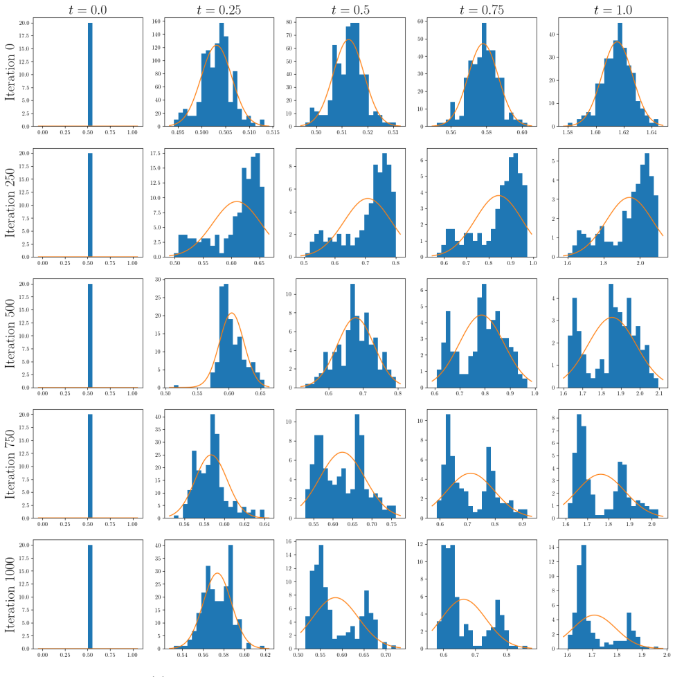
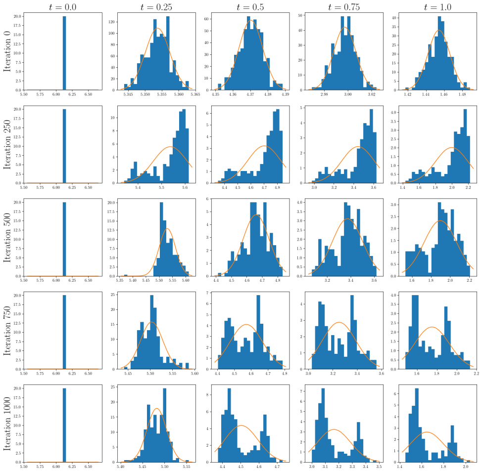
[Appendix I] The validation of the Gaussian likelihood assumption is not targeted at the quantity that matters. Appendix I examines the distribution of solutions uθ_det across training runs and overlays Gaussians with the sample mean and variance, but the likelihood in Eq. (17) concerns the conditional distribution of the error δ=u-uθ_det (or, in the two-step setup, the residual of the BNN fit). A histogram of solutions does not test whether the errors are Gaussian with scale B, nor whether the scale varies with x and lambda as claimed. The authors should provide direct diagnostics such as standardized residuals or quantile-quantile plots for δ/B, or at least explicitly acknowledge that the Gaussian assumption is an unverified modeling choice.
[Table 2 and Section 7] The caption of Table 2 states that metrics are computed in the 'Testing Region', but this region is never defined. Tables 3 and 4 separately consider training and OOD regions, and the choice of region can materially change the reported results; the catastrophic outliers in Table 13 for CPL and HS (e.g., 9.01e+08 and 3.88e+26) are not visible in Table 2, suggesting that the testing region excludes the most extreme points. Since the central claim that 'error bounds significantly enhance calibration' is based on Table 2, the authors must define the testing region precisely, report results on a fixed held-out set that includes all evaluation points, and explain how the OOD extremes are handled in the reported miscalibration areas.

minor comments (5)

[Table 2 caption] The phrase 'Testing Region' is undefined; please specify the exact domain and parameter ranges used for the evaluation.
[Appendix G.2, Eq. (51)] The expression for e^{P(z)} is printed twice with an apparent typo; the first line after 'we can then simplify' repeats the previous equation rather than showing the simplified form.
[Appendix J heading] The heading 'ADITIONAL RESULTS' should be 'ADDITIONAL RESULTS'.
[References] The reference to Hoffman and Gelman lacks publication details (year and venue), and several URLs in the reference list are incomplete or contain line breaks that may be artifacts of formatting.
[Section 4.3 and Table 2] The baseline residual-likelihood method is not implemented for NLM, and the paper does not discuss how the absence of NLM in the baseline affects the comparison; a brief comment would improve clarity.

Circularity Check

1 steps flagged · score 6.0 of 10

EB calibration gain is built in: σ_Like(x,λ)=B(x,λ) turns a worst-case error bound into a Gaussian noise scale, so the reported miscalibration-area improvement is an enclosure effect by construction.

self definitional [Section 2.6 (Eq. 11), Section 4.1 (Eq. 17), and Section 4.2 (Error Bounds Based Heteroscedastic option)]
"For the Solution Bundle setup, the network error is denoted as η(x,λ) := u(x,λ)−u~θ(x,λ), and the error bound is represented by a scalar function B such that ∥η(x,λ)∥≤ B(x,λ) (11) ... 2. Error Bounds Based Heteroscedastic: σLike(x,λ) = B(x,λ). This choice ensures we are taking into account the error made by uθ∗det in the predictive uncertainty."

The heteroscedastic likelihood variance is defined to be exactly B(x,λ), while Eq. (11) defines B as a worst-case upper bound on |u−uθdet| — an enclosure, not a statistical dispersion scale. Consequently, any predictive interval whose width is controlled by σLike=B must contain the deterministic solution essentially by theorem, so the observed reduction in miscalibration area for the EB variant is forced by the definition of σLike rather than by a validated Gaussian error model. The paper's own diagnostic in Appendix I checks the distribution of solutions, not the distribution of errors δ=u−uθdet, so it does not establish that residual errors are Gaussian with scale B. The central 'error bounds improve calibration' claim therefore reduces to the input property of B.

full rationale

The main circular step is the definitional identification σLike(x,λ)=B(x,λ), where B is a guaranteed (or intended) deterministic bound on |u−uθdet|. This makes improved calibration largely an enclosure artifact: intervals built from a worst-case bound cover the true solution by construction, independent of whether the Gaussian likelihood in Eq. (17) is correct. The paper also exhibits an object mismatch — Eq. (17) models the discrepancy uθdet−uθ as Gaussian noise with std B, whereas Eq. (11) bounds the different error u−uθdet; the transfer to BNN predictive intervals holds only if the BNN posterior mean coincides with uθdet, which is never checked and is contradicted in several OOD results. These are correctness risks, not additional circularities. The two-step training framework, the comparison against analytical/numerical solvers, and the inverse-problem pipeline against external cosmic-chronometer data are self-contained empirical work and are not circular. Self-citations to Liu et al. for the error bound and to Flamant et al. for Solution Bundles are load-bearing but are published prior results with stated assumptions; the decisive circularity is the equation-level reduction σLike=B, which forces the EB calibration gain.

Assumptions & free parameters 3 free parameters · 4 assumptions · 0 invented entities

The method's predictive uncertainty is built on a hand-chosen homoscedastic sigma_Like, or on B in the EB variant, a Gaussian likelihood assumption, and imported residual error bounds from prior work by the same group. No new physical entities are introduced. The key unvalidated step is the mapping B to sigma_Like.

free parameters (3)

homoscedastic likelihood standard deviation sigma_Like = 0.1 (LambdaCDM), 0.01 (CPL), 0.005 (Quintessence, HS)
Chosen per equation and per method in Tables 6-8; directly controls predictive width and calibration, with no data-driven selection criterion reported.
prior standard deviation sigma_prior = 1.0
Set for BBB and HMC in Tables 7-8; hand-chosen, affects posterior spread.
error-bound partition parameters N and K = not reported
Algorithm 1 requires the number of partitions N and points per partition K; their values determine tightness of B and are not stated for the experiments.

assumptions (4)

domain assumption Gaussian additive noise model in Eq. (17) captures the discrepancy between deterministic network output and BNN solution.
Section 4.1 assumes eta ~ N(0, sigma_Like) for tractability; the targets are deterministic PINN outputs, not noisy measurements, and Appendix I shows the actual solution distributions are only approximately Gaussian, with HS noticeably bimodal.
ad hoc to paper The residual-based upper bound B(x,lambda) can serve as the standard deviation of the likelihood.
Section 4.2 sets sigma_Like(x,lambda)=B(x,lambda); this equates a worst-case deterministic bound with a statistical dispersion scale, without derivation or coverage validation.
standard math Liu et al. residual error bounds for first-order linear ODEs are correct and applicable to LambdaCDM and CPL equations.
The paper imports these bounds in Section 2.6 and Appendix B; they are accepted from the cited literature and not re-derived.
domain assumption The deterministic PINN used in step one is accurate enough to serve as a target for BNN training.
The BNN is trained on u_theta_det outputs; if the deterministic network is poor in a region, the BNN inherits the error and the error bound B must cover it. The out-of-distribution results show this assumption can fail.

how reviews work

0 comments

Cite this review

Pith. "Pith review of Improved Uncertainty Quantification in Physics-Informed Neural Networks Using Error Bounds and Solution Bundles." pith.science (2026). https://pith.science/paper/HEH7TLLZ

@misc{pith2026250506459,
  author       = {Pith},
  title        = {Pith review of: Improved Uncertainty Quantification in Physics-Informed Neural Networks Using Error Bounds and Solution Bundles},
  year         = {2026},
  howpublished = {\url{https://pith.science/paper/HEH7TLLZ}},
  note         = {Machine review of arXiv:2505.06459}
}

read the original abstract

Physics-Informed Neural Networks (PINNs) have been widely used to obtain solutions to various physical phenomena modeled as Differential Equations. As PINNs are not naturally equipped with mechanisms for Uncertainty Quantification, some work has been done to quantify the different uncertainties that arise when dealing with PINNs. In this paper, we use a two-step procedure to train Bayesian Neural Networks that provide uncertainties over the solutions to differential equation systems provided by PINNs. We use available error bounds over PINNs to formulate a heteroscedastic variance that improves the uncertainty estimation. Furthermore, we solve forward problems and utilize the obtained uncertainties when doing parameter estimation in inverse problems in cosmology.

Figures

Figures reproduced from arXiv: 2505.06459 by the authors.

**Figure 2.** Diagram of Both Training Steps. In the Second [PITH_FULL_IMAGE:figures/full_fig_p005_2.png] view at source ↗

**Figure 3.** Examples of ΛCDM Bayesian Solutions Obtained Using the Bundle Solver. Analytic Solutions are Presented in Dotted Lines. to Eq. (20). This is the case in Section 4.1, where the dataset has observations uθ ∗ det (x, λ) free of noise: uθ ∗ det (x, λ) = uθ(x, λ) + ✁ ϵ + η (22) However, the approximate solution uθ ∗ det may still have prediction errors. We model this error with a Gaussian distribution with standard dev… view at source ↗

Figures from the paper (31 more)

**Figure 4.** Figure 4: Distribution of xm(z) from ΛCDM. Samples were collected as described in I. Orange lines show a Gaussian distribution with sample mean and variance [PITH_FULL_IMAGE:figures/full_fig_p022_4.png]

**Figure 5.** Figure 5: Distribution of xDE(z) from CPL. Samples were collected as described in I. Orange lines show a Gaussian distribution with sample mean and variance [PITH_FULL_IMAGE:figures/full_fig_p023_5.png]

**Figure 6.** Figure 6: Distribution of x(N) from Quintessence. Samples were collected as described in I. Orange lines show a Gaussian distribution with sample mean and variance [PITH_FULL_IMAGE:figures/full_fig_p024_6.png]

**Figure 7.** Figure 7: Distribution of y(N) from Quintessence. Samples were collected as described in I. Orange lines show a Gaussian distribution with sample mean and variance [PITH_FULL_IMAGE:figures/full_fig_p025_7.png]

**Figure 8.** Figure 8: Distribution of x(z) from HS. Samples were collected as described in I. Orange lines show a Gaussian distribution with sample mean and variance [PITH_FULL_IMAGE:figures/full_fig_p026_8.png]

**Figure 9.** Figure 9: Distribution of y(z) from HS. Samples were collected as described in I. Orange lines show a Gaussian distribution with sample mean and variance [PITH_FULL_IMAGE:figures/full_fig_p027_9.png]

**Figure 10.** Figure 10: Distribution of v(z) from HS. Samples were collected as described in I. Orange lines show a Gaussian distribution with sample mean and variance [PITH_FULL_IMAGE:figures/full_fig_p028_10.png]

**Figure 11.** Figure 11: Distribution of Ω(z) from HS. Samples were collected as described in I. Orange lines show a Gaussian distribution with sample mean and variance [PITH_FULL_IMAGE:figures/full_fig_p029_11.png]

**Figure 12.** Figure 12: Distribution of r(z) from HS. Samples were collected as described in I. Orange lines show a Gaussian distribution with sample mean and variance [PITH_FULL_IMAGE:figures/full_fig_p030_12.png]

**Figure 13.** Figure 13: Relationship Between Solution Errors and Residuals from [PITH_FULL_IMAGE:figures/full_fig_p031_13.png]

**Figure 14.** Figure 14: Relationship Between Solution Errors and Residuals from CPL. Samples were collected as described in I. [PITH_FULL_IMAGE:figures/full_fig_p031_14.png]

**Figure 15.** Figure 15: Relationship Between Solution Errors and Residuals from Quintessence. Samples were collected as described in [PITH_FULL_IMAGE:figures/full_fig_p031_15.png]

**Figure 16.** Figure 16: Relationship Between Solution Errors and Residuals from HS. Samples were collected as described in I. Colors [PITH_FULL_IMAGE:figures/full_fig_p032_16.png]

**Figure 17.** Figure 17: ΛCDM Bayesian Solutions. The Analytic Solution Is Presented In Dotted Lines [PITH_FULL_IMAGE:figures/full_fig_p034_17.png]

**Figure 18.** Figure 18: ΛCDM Bayesian Solutions With Error Bounds. The Analytic Solution Is Presented In Dotted Lines [PITH_FULL_IMAGE:figures/full_fig_p034_18.png]

**Figure 19.** Figure 19: CPL Bayesian Solutions. The Analytic Solution Is Presented In Dotted Lines. [PITH_FULL_IMAGE:figures/full_fig_p034_19.png]

**Figure 20.** Figure 20: CPL Bayesian Solutions With Error Bounds. The Analytic Solution Is Presented In Dotted Lines. [PITH_FULL_IMAGE:figures/full_fig_p035_20.png]

**Figure 21.** Figure 21: Quintessence Bayesian Solutions Residual Likelihood. The Numerical Solution Is Presented In Dotted Lines. [PITH_FULL_IMAGE:figures/full_fig_p035_21.png]

**Figure 22.** Figure 22: Quintessence Bayesian Solutions. The Numerical Solution Is Presented In Dotted Lines. [PITH_FULL_IMAGE:figures/full_fig_p036_22.png]

**Figure 23.** Figure 23: HS Bayesian solutions Residual Likelihood. The Numerical Solution Is Presented In Dotted Lines. [PITH_FULL_IMAGE:figures/full_fig_p037_23.png]

**Figure 24.** Figure 24: HS Bayesian solutions. The Numerical Solution Is Presented In Dotted Lines. [PITH_FULL_IMAGE:figures/full_fig_p038_24.png]

**Figure 25.** Figure 25: Examples Of CPL Bayesian Solutions Obtained Using The Bundle Solver. Analytic Solutions Are Presented In [PITH_FULL_IMAGE:figures/full_fig_p039_25.png]

**Figure 26.** Figure 26: Examples Of CPL Bayesian Solutions Obtained Using The Bundle Solver With Error Bounds. Analytic Solutions [PITH_FULL_IMAGE:figures/full_fig_p040_26.png]

**Figure 27.** Figure 27: Examples of Quintessence Bayesian Solutions Obtained Using The Bundle Solver For The Parameter Value [PITH_FULL_IMAGE:figures/full_fig_p040_27.png]

**Figure 28.** Figure 28: Examples of Quintessence Bayesian Solutions Obtained Using The Bundle Solver For The Parameter Value [PITH_FULL_IMAGE:figures/full_fig_p041_28.png]

**Figure 29.** Figure 29: Examples of Quintessence Bayesian Solutions Obtained Using The Bundle Solver For The Parameter Value [PITH_FULL_IMAGE:figures/full_fig_p041_29.png]

**Figure 30.** Figure 30: Examples of Quintessence Bayesian Solutions Obtained Using The Bundle Solver For The Parameter Value [PITH_FULL_IMAGE:figures/full_fig_p042_30.png]

**Figure 31.** Figure 31: Examples Of HS Bayesian Solutions Obtained Using The Bundle Solver For The Parameter Value [PITH_FULL_IMAGE:figures/full_fig_p043_31.png]

**Figure 32.** Figure 32: Examples Of HS Bayesian Solutions Obtained Using The Bundle Solver For The Parameter Value [PITH_FULL_IMAGE:figures/full_fig_p044_32.png]

**Figure 33.** Figure 33: Examples Of HS Bayesian Solutions Obtained Using The Bundle Solver For The Parameter Value [PITH_FULL_IMAGE:figures/full_fig_p045_33.png]

**Figure 34.** Figure 34: Examples Of HS Bayesian Solutions Obtained Using The Bundle Solver For The Parameter Value [PITH_FULL_IMAGE:figures/full_fig_p046_34.png]

Discussion (0). Continue with ORCID to comment.

Reference graph

Works this paper leans on

12 extracted references · 3 canonical work pages

[1]

Zhang Cong, Zhang Han, Yuan Shuo, Liu Siqi, Zhang Tong-Jie, and Sun Yan-Chun

URL https://www.sciencedirect.com/ science/article/pii/S0370157312000105. Zhang Cong, Zhang Han, Yuan Shuo, Liu Siqi, Zhang Tong-Jie, and Sun Yan-Chun. Four new observa- tional H(z) data from luminous red galaxies in the Sloan Digital Sky Survey data release seven. Research in Astronomy and Astrophysics , 14(10):1221, October

work page
[11]

doi: 10.1029/2021JB023120

ISSN 2169-9356. doi: 10.1029/2021JB023120. URL https://onlinelibrary.wiley.com/ doi/abs/10.1029/2021JB023120. _eprint: https://onlinelibrary.wiley.com/doi/pdf/10.1029/2021JB023120. Joan Simon, Licia Verde, and Raul Jimenez. Con- straints on the redshift dependence of the dark energy potential. Physical Review D , 71(12): 123001, June 2005. doi: 10.1103/Ph...

arXiv
[12]

consists of a system of 5 equations. dx dz = 1 z + 1(−Ω− 2v +x + 4y +xv +x2) dy dz = −1 z + 1(vxΓ−xy + 4y− 2yv) dv dz = −v z + 1(xΓ + 4− 2v) dΩ dz = Ω z + 1(−1 + 2v +x) dr dz =− rΓx z + 1 where Γ(r) = (r +b) (r +b)2− 2b 4br The initial conditions are x0 = 0 y0 = ΩΛ m,0(1 +z0)3 + 2(1− ΩΛ m,0) 2 ΩΛ m,0(1 +z0)3 + (1− ΩΛ m,0) v0 = ΩΛ m,0(1 +z0)3 + 4(1− ΩΛ m,0...

work page arXiv 2022
[45]

Majid Rasht-Behesht, Christian Huber, Khemraj Shukla, and George Em Karniadakis

URL https://www.sciencedirect.com/ science/article/pii/S0021999118307125. Majid Rasht-Behesht, Christian Huber, Khemraj Shukla, and George Em Karniadakis. Physics-Informed Neural Networks (PINNs) for Wave Propagation and Full Waveform Inversions. Journal of Geophysi- cal Research: Solid Earth , 127(5):e2021JB023120,

work page
[2007]

URL https://link.aps.org/doi/10.1103/ PhysRevD.76.064004

doi: 10.1103/PhysRevD.76.064004. URL https://link.aps.org/doi/10.1103/ PhysRevD.76.064004. Publisher: American Physical Society. Xiaowei Jin, Shengze Cai, Hui Li, and George Em Karniadakis. NSFnets (Navier-Stokes flow nets): Physics-informed neural networks for the incom- pressible Navier-Stokes equations. Journal of Computational Physics , 426:109951, Fe...

arXiv
[2014]

doi: 10.1088/1674-4527/14/ 10/002

ISSN 1674-4527. doi: 10.1088/1674-4527/14/ 10/002. URL https://dx.doi.org/10.1088/ 1674-4527/14/10/002. Edmund J. Copeland, Andrew R. Liddle, and David Wands. Exponential potentials and cosmological scaling solutions. Physical Review D , 57(8):4686– 4690, April 1998. doi: 10.1103/PhysRevD.57.4686. URL https://link.aps.org/doi/10.1103/ PhysRevD.57.4686. Pu...

arXiv
[2019]

doi: 10.1016/j.jcp.2018.10

ISSN 0021-9991. doi: 10.1016/j.jcp.2018.10

doi:10.1016/j.jcp.2018.10 2018
[2021]

doi: 10.1111/mice.12685

ISSN 1467-8667. doi: 10.1111/mice.12685. URL https://onlinelibrary.wiley.com/ doi/abs/10.1111/mice.12685. _eprint: https://onlinelibrary.wiley.com/doi/pdf/10.1111/mice.12685. Adam Paszke, Sam Gross, Francisco Massa, Adam Lerer, James Bradbury, Gregory Chanan, Trevor Killeen, Zem- ing Lin, Natalia Gimelshein, Luca Antiga, Alban Des- maison, Andreas Köpf, E...

arXiv

Show all 12 references

[2022]

URL http://arxiv.org/abs/2207. 01114. arXiv:2207.01114 [cs, math]. Shuheng Liu, Xiyue Huang, and Pavlos Protopapas. Residual-based error bound for physics-informed neu- ral networks. June 2023. Zhiping Mao, Ameya D. Jagtap, and George Em Kar- niadakis. Physics-informed neural ...

2023 arXiv
[3978]

URL http:// arxiv.org/abs/1808.09440

doi: 10.1002/prop.201800075. URL http:// arxiv.org/abs/1808.09440. arXiv:1808.09440 [astro-ph, physics:gr-qc, physics:hep-ph, physics:hep-th, physics:math-ph]. C. Armendariz-Picon, V . Mukhanov, and Paul J. Stein- hardt. Dynamical Solution to the Problem of a Small Cosmologica...

arXiv
[4438]

1103/PhysRevLett.85.4438

URL https://link.aps.org/doi/10. 1103/PhysRevLett.85.4438. Publisher: Ameri- can Physical Society. Eli Bingham, Jonathan P. Chen, Martin Jankowiak, Fritz Obermeyer, Neeraj Pradhan, Theofanis Karaletsos, Rohit Singh, Paul Szerlip, Paul Horsfall, and Noah D. Goodman. Pyro: Deep ...

arXiv
[9044]

URL https: //doi.org/10.1007/s10444-022-09985-9

doi: 10.1007/s10444-022-09985-9. URL https: //doi.org/10.1007/s10444-022-09985-9 . Tim De Ryck and Siddhartha Mishra. Generic bounds on the approximation error for physics-informed (and) operator learning. May 2022b. URL https://openreview. net/forum?id=bF4eYy3LTR9. Tim De Ryc...

arXiv

Pith tools

Reviewed August 15, 2026 · model on record in the stance chip above.

[1] [1]

Zhang Cong, Zhang Han, Yuan Shuo, Liu Siqi, Zhang Tong-Jie, and Sun Yan-Chun

URL https://www.sciencedirect.com/ science/article/pii/S0370157312000105. Zhang Cong, Zhang Han, Yuan Shuo, Liu Siqi, Zhang Tong-Jie, and Sun Yan-Chun. Four new observa- tional H(z) data from luminous red galaxies in the Sloan Digital Sky Survey data release seven. Research in Astronomy and Astrophysics , 14(10):1221, October

work page

[2] [11]

doi: 10.1029/2021JB023120

ISSN 2169-9356. doi: 10.1029/2021JB023120. URL https://onlinelibrary.wiley.com/ doi/abs/10.1029/2021JB023120. _eprint: https://onlinelibrary.wiley.com/doi/pdf/10.1029/2021JB023120. Joan Simon, Licia Verde, and Raul Jimenez. Con- straints on the redshift dependence of the dark energy potential. Physical Review D , 71(12): 123001, June 2005. doi: 10.1103/Ph...

arXiv

[3] [12]

consists of a system of 5 equations. dx dz = 1 z + 1(−Ω− 2v +x + 4y +xv +x2) dy dz = −1 z + 1(vxΓ−xy + 4y− 2yv) dv dz = −v z + 1(xΓ + 4− 2v) dΩ dz = Ω z + 1(−1 + 2v +x) dr dz =− rΓx z + 1 where Γ(r) = (r +b) (r +b)2− 2b 4br The initial conditions are x0 = 0 y0 = ΩΛ m,0(1 +z0)3 + 2(1− ΩΛ m,0) 2 ΩΛ m,0(1 +z0)3 + (1− ΩΛ m,0) v0 = ΩΛ m,0(1 +z0)3 + 4(1− ΩΛ m,0...

work page arXiv 2022

[4] [45]

Majid Rasht-Behesht, Christian Huber, Khemraj Shukla, and George Em Karniadakis

URL https://www.sciencedirect.com/ science/article/pii/S0021999118307125. Majid Rasht-Behesht, Christian Huber, Khemraj Shukla, and George Em Karniadakis. Physics-Informed Neural Networks (PINNs) for Wave Propagation and Full Waveform Inversions. Journal of Geophysi- cal Research: Solid Earth , 127(5):e2021JB023120,

work page

[5] [2007]

URL https://link.aps.org/doi/10.1103/ PhysRevD.76.064004

doi: 10.1103/PhysRevD.76.064004. URL https://link.aps.org/doi/10.1103/ PhysRevD.76.064004. Publisher: American Physical Society. Xiaowei Jin, Shengze Cai, Hui Li, and George Em Karniadakis. NSFnets (Navier-Stokes flow nets): Physics-informed neural networks for the incom- pressible Navier-Stokes equations. Journal of Computational Physics , 426:109951, Fe...

arXiv

[6] [2014]

doi: 10.1088/1674-4527/14/ 10/002

ISSN 1674-4527. doi: 10.1088/1674-4527/14/ 10/002. URL https://dx.doi.org/10.1088/ 1674-4527/14/10/002. Edmund J. Copeland, Andrew R. Liddle, and David Wands. Exponential potentials and cosmological scaling solutions. Physical Review D , 57(8):4686– 4690, April 1998. doi: 10.1103/PhysRevD.57.4686. URL https://link.aps.org/doi/10.1103/ PhysRevD.57.4686. Pu...

arXiv

[7] [2019]

doi: 10.1016/j.jcp.2018.10

ISSN 0021-9991. doi: 10.1016/j.jcp.2018.10

doi:10.1016/j.jcp.2018.10 2018

[8] [2021]

doi: 10.1111/mice.12685

ISSN 1467-8667. doi: 10.1111/mice.12685. URL https://onlinelibrary.wiley.com/ doi/abs/10.1111/mice.12685. _eprint: https://onlinelibrary.wiley.com/doi/pdf/10.1111/mice.12685. Adam Paszke, Sam Gross, Francisco Massa, Adam Lerer, James Bradbury, Gregory Chanan, Trevor Killeen, Zem- ing Lin, Natalia Gimelshein, Luca Antiga, Alban Des- maison, Andreas Köpf, E...

arXiv