REVIEW 3 major objections 5 minor 1 cited by
Coherent injection of magnetic noise and its impact on gravitational-wave searches
T0 review · 3 major / 5 minor · reviewed 2026-08-15 · deepseek-v4-flash
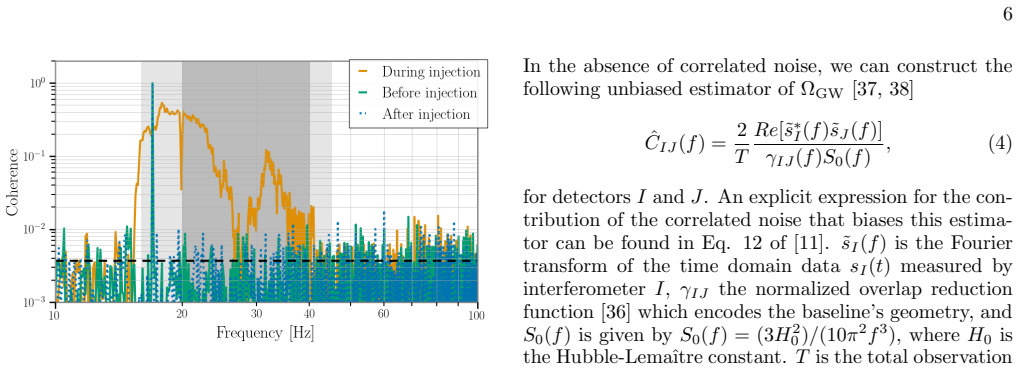
Pith's one-line read The first coherent broadband magnetic noise injection between two gravitational-wave detectors created measurable strain-strain coherence between about 16 and 40 Hz, and a single-magnetometer Wiener filter removed it.
desk verdict A genuinely new inter-site coherent magnetic noise injection with a solid projection comparison; the Wiener-filter conclusion overreaches and needs revision. read the letter →
The pith
A machine-rendered reading of the paper's core claim, the machinery that carries it, and where it could break.
The reading
What carries the argument
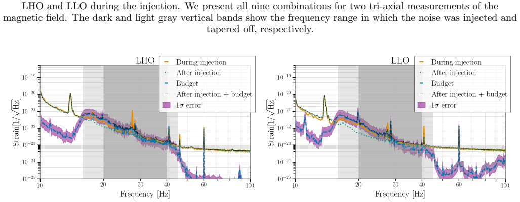
The central object is the coherent injection itself: the same prescribed broad-band magnetic spectrum, modelled on Schumann resonances observed at Sos Enattos and tapered to 16-42 Hz, played out synchronously through large injection coils at each central station. The argument is carried by the comparison between the observed magnetometer-to-magnetometer coherence and the strain-to-strain coherence, and by two transfer tools: the O4a magnetic coupling functions $\kappa_I(f)$ used to project magnetic ASD into strain ASD, and the Wiener filter $\kappa_{I,\mathrm{Wiener}} = \langle s_I w_I\rangle/\langle w_I w_I\rangle$ estimated from one witness channel. The magnetic cross-correlation statistic of Eq. (6) connects the two, and the crucial limitation is that only the magnitude of $\kappa_I$ is known, so the phase of the coupling is left out of the projection.
What would settle it
Measure the complex transfer function from injected coil current to strain at each site across 16-42 Hz. If the phase difference between Hanford and Livingston is nonzero and grows just where the real-part strain CSD drops, the paper's explanation holds; if the phase difference is zero, the over-projection would have to come from something else, such as the quadrature-sum method or unmodelled amplitude changes.
Extended reading notes
Core claim
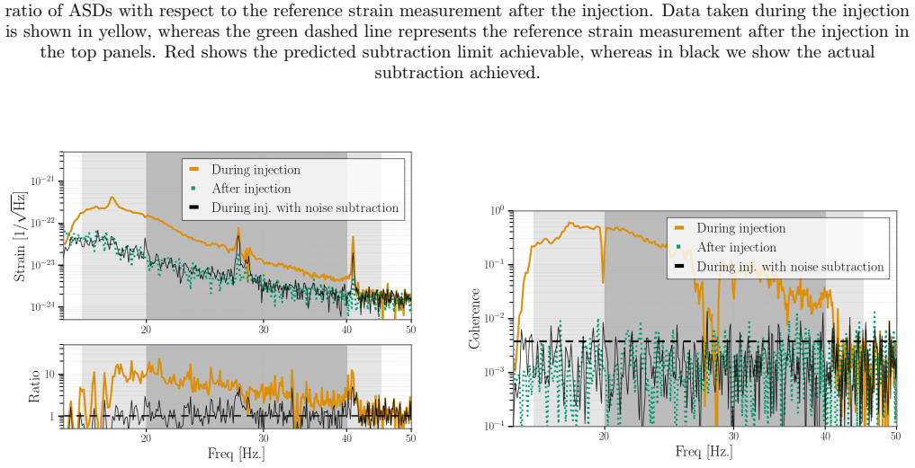
The central claim is that the December 20, 2023 injection succeeded: it produced coherent magnetic fields at both sites, and the resulting strain-strain coherence between 16 and 40 Hz is attributable to the injected magnetic field. Projecting the observed tri-axial magnetic noise through the O4a coupling functions reproduces the magnitude of the strain effect within about a factor of two, though it overestimates the correlated strain above roughly 30 Hz because the coupling functions carry no phase information and the true coupling phase differs between sites. Running the data through the isotropic background search pipeline recovers a loud, steep power-law signal with spectral index around -10.2, as expected if the correlated magnetic noise were a foreground. Finally, a time-domain Wiener filter using one vertex magnetometer as a witness removes essentially all of the correlated strain noise, restoring the ASD and CSD to reference levels, with the caveat that the subtraction leaves residual effects visible in the background search at the 3-4 sigma level.
Load-bearing premise
The projection rests on treating the O4a magnetic-to-strain coupling functions as still valid and as carrying no phase, when the data itself indicates the coupling phase is site-dependent and nonzero above about 30 Hz.
Editorial extensions
If this is right
- Correlated magnetic noise of the kind produced here would appear in an isotropic gravitational-wave background search as a steep, loud power-law signal; in this dataset the recovered spectral index is about -10.2, far steeper than any expected astrophysical background, so spectral separation should be possible.
- The quadrature sum over all nine magnetometer orientation pairs overestimates the true correlated magnetic contribution by about a factor of two.
- A single magnetometer witness at the same site, processed through a time-domain Wiener filter, can remove essentially all of the correlated broadband magnetic noise from the strain channel and restore the strain CSD to reference levels.
- Noise subtraction is not risk-free: the background search on the subtracted data shows residual structure, such as a 3.45 sigma feature with spectral index about 1.5, so Wiener filtering should be applied with caution in real searches.
- Because the coupling phase differs between sites and is not captured by current magnitude-only coupling functions, future noise projections should measure and include the phase of the magnetic-to-strain transfer function.
Reading between the lines
- Editorial inference: The same experiment design, repeated with injection amplitude below the strain ASD floor but high enough to accumulate in cross-correlation, would directly test how Wiener filtering behaves in the realistic sub-threshold regime the authors flag as untested.
- Editorial inference: The phase decorrelation above about 30 Hz implies that a network of three or more sites could, in principle, distinguish a common Schumann-type magnetic foreground from a genuine gravitational-wave background by comparing the phase structure of the cross-spectra across baselines.
- Editorial inference: The authors' finding that subtraction leaves residual spectral-index structure suggests that any Wiener-filter-based cleaning pipeline should be validated end-to-end with the same background-search statistic it is meant to protect, not just by ASD and CSD agreement.
Signed reviews
Editorial analysis
A structured set of objections, weighed in public.
Referee Report
Summary. The manuscript reports the first coherent broadband magnetic-noise injection performed simultaneously at LIGO Hanford and LIGO Livingston, using synchronized injection coils to create correlated magnetic fields across ~3000 km. The authors characterize the injected magnetic field at multiple witness sensors, show that the injection produces significant strain-strain coherence between roughly 16 and 40 Hz, and compare the observed correlated strain with noise projections built from the independently measured O4a magnetic coupling functions. They then analyze the data with the LVK isotropic GWB search pipeline (pygwb), finding a loud power-law signal with a steep spectral index. Finally, they apply a time-domain Wiener filter using a single magnetometer as a witness, demonstrating that the injected noise can be strongly suppressed in the ASD and CSD, but they also report residual artifacts in the subsequent GWB analysis. The paper concludes that Wiener filtering is effective and can be applied in future GWB searches, while cautioning that the method may alter the data in unforeseen ways.
Significance. The experimental accomplishment is substantial: creating a controlled, coherent, broadband magnetic field across two widely separated gravitational-wave detectors and observing its coupling into the strain channel provides a unique testing ground for correlated-noise projection and subtraction methods that are central to future GWB searches. The noise projections use coupling functions measured in an independent O4a injection campaign, which avoids the circularity that often plagues witness-channel studies. The paper is also refreshingly honest about the limitations it uncovers, including the >1-sigma overestimation of the correlated magnetic budget and the non-negligible phase of the magnetic-to-strain coupling. The dataset and the analysis results will be valuable for future studies of Schumann-resonance noise and for developing spectral-separation techniques. However, the abstract's strong claim that Wiener filtering is 'effective and can be applied' to GWB detection goes beyond what the current in-sample, high-amplitude demonstration establishes, given the residual artifacts reported in the subtracted-data GWB analysis.
major comments (3)
- [Sec. VI.A, Eq. (12)] The Wiener-filter demonstration is an in-sample test: the filter coefficients κ_I,Wiener are computed from the full 43-minute noise-injection dataset using Eq. (12), and the suppression is then evaluated on the same dataset. The clean recovery of the reference ASD and CSD in Figs. 10 and 11 therefore does not demonstrate that the filter generalizes to independent data, where the SNR of the magnetic signal in the witness channel will be much lower. An out-of-sample evaluation—for example, training on one half of the injection segment and testing on the other, or training on the injection segment and testing on a separate time with similar coupling—is needed to support the claim that the method is applicable to realistic GWB searches.
- [Sec. VI.B, Table II, and Sec. VII] The noise-subtracted data still contain substantial artifacts in the GWB analysis: the zero-lag result shows a 3.45-sigma excess at α=1.5 and a signal-to-noise ratio of -7.32 at α=-10.2, and the text in Sec. VII concedes that the filter 'might alter the data in unknown and unforeseen ways.' These residuals are not negligible for a search aiming at a 5-sigma detection, and they show that the subtraction is not simply removing the correlated noise without side effects. The abstract's final sentence, which states that Wiener filtering is effective and can be applied in the eventual detection of the GWB, is therefore not supported by the evidence presented; at most, the paper demonstrates a proof-of-concept that requires further validation with lower-amplitude injections and out-of-sample tests.
- [Sec. IV, Eq. (6), Fig. 7] The comparison between the projected and observed correlated strain relies on coupling functions that are measured in amplitude only, while Eq. (6) uses the real part of the magnetic CSD. The paper itself notes that the phase of the magnetic-to-strain coupling appears to be site-dependent and non-zero, particularly above 30 Hz, and that this leads to a systematic overestimation of the projection. Because the phase is not characterized, the quantitative agreement between the projection and the observed strain-strain coherence cannot be fully assessed. This is an acknowledged limitation rather than a hidden flaw, but it should be stated more prominently in the abstract or introduction: the injection demonstrates the existence of coherent magnetic coupling, but the accuracy of the projection method remains uncertain at the level set by the >1-sigma discrepancy shown in Fig. 7.
minor comments (5)
- [Sec. IV, Eq. (7)] There is a typo in the sentence introducing Eq. (7): 'detectror I' should be 'detector I'. Additionally, 'concretly' in the following paragraph should be 'concretely'.
- [Sec. V, Fig. 9] The corner plot in Fig. 9 shows a posterior for α that is quite broad; the text should state more explicitly whether this is consistent with the injected spectrum, since the injected signal has a known, non-power-law shape. This would help the reader connect the injected spectrum to the recovered spectral index.
- [Sec. VI.A] When describing the high-pass filter, the text notes that an 8th-order Butterworth filter with a cutoff of 16 Hz is applied, but it does not specify whether the same filter is applied to the witness channel before computing Eq. (12). If the witness is filtered differently, the transfer function should be described, as it affects the meaning of the Wiener filter coefficients.
- [Sec. VI.B] The text states that 'reweighting the frequentist results to α=1.5' gives a point estimate and standard deviation, but Table II does not list the α=1.5 row. Please add this row or clarify in the text, since the reader needs to see the numbers directly.
- [Sec. II.B] The coil-field distance estimate using Eq. (2) neglects the coil radius and the square geometry; the text acknowledges this, but it would be helpful to state the expected uncertainty on the ratio (e.g., factor of 2) so the reader can judge how well the observed 8:1 ratio matches the model.
Circularity Check
The Wiener-filter 'effectiveness' claim is supported by a filter trained and evaluated on the same injection dataset, while the magnetic projections rely on independent O4a coupling functions.
-
fitted input called prediction
[Sec. VI.A, Eq. (12), Figs. 10-11; abstract]
"For this demonstration we used the entire noise dataset to train our Wiener filter using 100 second windows. ... We conclude the time-based Wiener filter using one witness channel is able to reach, and in some frequency regions even outperform, its predicted subtraction limit based on the coherence between witness and target channels."
Equation (12) estimates kappa_I,Wiener = <s_I w_I>/<w_I w_I> from the same 43-minute injection data that is then subtracted and displayed in Figs. 10-11. Because the Wiener filter minimizes the in-sample mean-square residual, the observed reduction of the ASD/CSD toward the quiet reference is, to first order, the objective being optimized rather than an independent prediction. The abstract's conclusion that 'Wiener filtering is effective and can be applied' therefore converts this training-set demonstration into a general result without a held-out segment or independently estimated filter.
full rationale
The magnetic budget and GWB projections in Secs. III-IV are not circular: they multiply the measured magnetometer ASD/CSD by coupling functions from the separate O4a injection campaign (refs. [20,35]) and compare the result to strain data, so the comparison is not an identity. The phase-free coupling assumption is an acknowledged limitation, not a circular step. The only construction-like step is the Wiener-filter showcase in Sec. VI.A, where the filter is trained on the entirety of the injection data and the same data are used to display the subtracted ASD/CSD; the paper itself flags the in-sample and high-amplitude character ('proof-of-concept', 'entire noise dataset', and Sec. VII's warning that the filter 'might alter the data in unknown and unforeseen ways'). This limits the damage but does not remove the fact that the abstract's unqualified 'can be applied' statement rests on a training-set fit. No load-bearing self-citation chain is present: the O4a coupling measurements are independent empirical inputs, and the other self-citations are methodological rather than derivational.
Assumptions & free parameters
free parameters (4)
- Injection amplitude scaling =
O(10^4) times ambient Schumann spectrum near Vertex
- Injected spectral taper slopes =
f^3 below 18 Hz, f^-2.5 above 42 Hz
- Butterworth filter parameters =
32nd-order high-pass at 16 Hz, 32nd-order low-pass at 42 Hz
- Wiener filter coefficients =
computed from the full injection dataset via Eq. (12)
assumptions (5)
- domain assumption The O4a magnetic coupling functions kappa(f) remain valid for the December 2023 injection.
- domain assumption The magnetic coupling is linear and the strain signal is s = h + n + kappa*m (Eq. 10).
- domain assumption Witness sensor data is w = eta + m, with eta independent of m and of the strain noise.
- domain assumption Detector noise between sites is uncorrelated: <n_I n_J> = 0.
- standard math The GWB cross-correlation statistic's variance formula (Eq. 5) holds.
Cite this review
Pith. "Pith review of Coherent injection of magnetic noise and its impact on gravitational-wave searches." pith.science (2026). https://pith.science/paper/YAJ6J4UE
@misc{pith2026250511903,
  author       = {Pith},
  title        = {Pith review of: Coherent injection of magnetic noise and its impact on gravitational-wave searches},
  year         = {2026},
  howpublished = {\url{https://pith.science/paper/YAJ6J4UE}},
  note         = {Machine review of arXiv:2505.11903}
}
read the original abstract
Correlated noise sources, particularly magnetic noise, form a risk to future gravitational-wave searches aimed at detecting the gravitational-wave background. Potential noise contamination is investigated by making noise projections which typically rely on an accurate measurement of the coupling strength of the noise to the detector. To make these projections, we inject, for the first time, broadband, coherent magnetic noise between two gravitational-wave detectors, LIGO Hanford and LIGO Livingston, separated by several thousands of kilometers. We describe the noise injection as well as its impact on the analysis pipelines and investigate the accuracy of noise projection techniques used in the past decade. Finally, we present a proof-of-concept demonstration of noise subtraction using Wiener filtering, while also highlighting potential risks associated with this method. This unique data set with correlated noise caused by magnetic field fluctuations in two gravitational-wave detectors, as well as in an array of witness sensors, provides an excellent testing ground for additional future studies. Ultimately, this study demonstrates that Wiener filtering is effective and can be applied in the eventual detection of the gravitational-wave background by the LIGO-Virgo-KAGRA Collaboration.
Figures


Figures from the paper (11 more)





Forward citations
Cited by 1 Pith paper
-
LIGO Detector Characterization in the Second and Third Parts of the Fourth Observing Run
This is the archival record of LIGO noise hunting, hardware repairs, event validation, and data quality products for the O4b and O4c observing periods.
Reference graph
Works this paper leans on
-
[1]
Aasiet al., Classical and Quantum Gravity32, 074001 (2015)
J. Aasiet al., Classical and Quantum Gravity32, 074001 (2015)
2015
-
[2]
Acerneseet al.(Virgo Collaboration), Class
F. Acerneseet al.(Virgo Collaboration), Class. Quant. Grav.32, 024001 (2015), arXiv:1408.3978 [gr-qc]
arXiv 2015
-
[3]
Y. Aso, Y. Michimura, K. Somiya, M. Ando, O. Miyakawa, T. Sekiguchi, D. Tatsumi, and H. Ya- mamoto (The KAGRA Collaboration), Phys. Rev. D88, 043007 (2013)
work page 2013
-
[4]
Christensen, Reports on Progress in Physics82, 016903 (2018)
N. Christensen, Reports on Progress in Physics82, 016903 (2018)
2018
- [5]
- [6]
-
[7]
Here we notice that the correlated power starts to de- crease just before 30Hz and predicts lower contributions between 30Hz and 40Hz compared to the absolute value of the strain-strain CSD. However, a similar behaviour is not observed for the magnetic budget using the real part of the magnetic CSDs. This seems to indicate there is an induced phase differ...
-
[8]
M. W. Coughlinet al., Class. Quant. Grav.33, 224003 (2016), arXiv:1606.01011 [gr-qc]
arXiv 2016
Show all 40 references
-
[9]
Himemoto and A
Y. Himemoto and A. Taruya, Phys. Rev. D96, 022004 (2017)
2017
-
[10]
M. W. Coughlin, A. Cirone, P. Meyers, S. Atsuta, V. Boschi, A. Chincarini, N. L. Christensen, R. De Rosa, A. Effler, I. Fiori, M. Go lkowski, M. Guidry, J. Harms, K. Hayama, Y. Kataoka, J. Kubisz, A. Kulak, M. Laxen, A. Matas, J. Mlynarczyk, T. Ogawa, F. Paoletti, J. Sal- vado...
2018
-
[11]
Himemoto and A
Y. Himemoto and A. Taruya, Phys. Rev. D100, 082001 (2019)
2019
-
[12]
P. M. Meyers, K. Martinovic, N. Christensen, and M. Sakellariadou, Phys. Rev. D102, 102005 (2020), arXiv:2008.00789 [gr-qc]
2020 arXiv
-
[13]
Janssens, K
K. Janssens, K. Martinovic, N. Christensen, P. M. Mey- ers, and M. Sakellariadou, Phys. Rev. D104, 122006 (2021)
2021
-
[14]
Janssens, M
K. Janssens, M. Ball, R. M. S. Schofield, N. Christensen, R. Frey, N. van Remortel, S. Banagiri, M. W. Coughlin, A. Effler, M. Go lkowski, J. Kubisz, and M. Ostrowski, Phys. Rev. D107, 022004 (2023)
2023
-
[15]
Janssens, G
K. Janssens, G. Boileau, N. Christensen, F. Badaracco, and N. van Remortel, Phys. Rev. D106, 042008 (2022)
2022
-
[16]
W. O. Schumann, Zeitschrift Naturforschung Teil A7, 149 (1952)
1952
-
[17]
W. O. Schumann, Zeitschrift Naturforschung Teil A7, 250 (1952)
1952
-
[18]
Venikoudis, F
S. Venikoudis, F. De Lillo, K. Janssens, J. Suresh, and G. Bruno, Phys. Rev. D111, 082005 (2025)
2025
-
[19]
Fiori, F
I. Fiori, F. Paoletti, M. C. Tringali, K. Janssens,et al., Galaxies8(2020), 10.3390/galaxies8040082
2020 doi
-
[20]
Nguyenet al., Classical and Quantum Gravity38, 145001 (2021)
P. Nguyenet al., Classical and Quantum Gravity38, 145001 (2021)
2021
-
[21]
Soniet al., Classical and Quantum Gravity42, 085016 (2025)
S. Soniet al., Classical and Quantum Gravity42, 085016 (2025)
2025
-
[22]
Punturo, M
M. Punturo, M. Abernathy, F. Acernese,et al., Classical and Quantum Gravity27, 194002 (2010)
2010
-
[23]
Hildet al., Class
S. Hildet al., Class. Quant. Grav.28, 094013 (2011), arXiv:1012.0908 [gr-qc]
2011 arXiv
-
[24]
Maggiore, C
M. Maggiore, C. V. D. Broeck, N. Bartolo, E. Belgacem, D. Bertacca, M. A. Bizouard, M. Branchesi, S. Clesse, S. Foffa, J. Garc´ ıa-Bellido, S. Grimm, J. Harms, T. Hin- derer, S. Matarrese, C. Palomba, M. Peloso, A. Ricciar- done, and M. Sakellariadou, Journal of Cosmology and ...
2020
-
[25]
Amannet al., Rev
F. Amannet al., Rev. Sci. Instrum.91, 9 (2020), arXiv:2003.03434 [physics.ins-det]
2020 arXiv
-
[26]
ET Steering Committee Editorial Team, (2020), ET- 0007B-20
2020
-
[27]
Reitze, R
D. Reitze, R. X. Adhikari, S. Ballmer, B. Barish, L. Bar- sotti, G. Billingsley, D. A. Brown, Y. Chen, D. Coyne, R. Eisenstein, M. Evans, P. Fritschel, E. D. Hall, A. Laz- zarini, G. Lovelace, J. Read, B. S. Sathyaprakash, D. Shoemaker, J. Smith, C. Torrie, S. Vitale, R. Weiss...
2019
-
[28]
Kowalska-Leszczynska, I et al, Classical and Quantum Gravity34, 074002 (2017)
2017
-
[29]
Abbott, T
R. Abbott, T. D. Abbott, S. Abraham,et al.(LIGO Sci- entific Collaboration, Virgo Collaboration, and KAGRA Collaboration), Phys. Rev. D104, 022004 (2021)
2021
-
[30]
A. I. Renziniet al., Astrophys. J.952, 25 (2023), arXiv:2303.15696 [gr-qc]
2023 arXiv
-
[31]
aLIGO LHO Logbook,
J. Driggers, “aLIGO LHO Logbook,” Available at https://alog.ligo-wa.caltech.edu/aLOG/index.php? callRep=70916(2023)
2023
-
[32]
aLIGO LLO Logbook,
J. Betzwieser, “aLIGO LLO Logbook,” Available at https://alog.ligo-la.caltech.edu/aLOG/index.php? callRep=65938(2023)
2023
-
[33]
aLIGO LHO Logbook,
J. Driggers, “aLIGO LHO Logbook,” Available at https://alog.ligo-wa.caltech.edu/aLOG/index.php? callRep=74941(2023). 14
2023
-
[34]
aLIGO LLO Logbook,
J. Betzwieser, “aLIGO LLO Logbook,” Available at https://alog.ligo-la.caltech.edu/aLOG/index.php? callRep=68845(2023)
2023
-
[35]
D. J. Griffiths,Introduction to Electrodynamics(Prentice Hall, 1999)
1999
-
[36]
A. F. Helmling-Cornell, P. Nguyen, R. M. S. Schofield, and R. Frey, Classical and Quantum Gravity41, 145003 (2024), arXiv:2312.00735 [gr-qc]
2024 arXiv
-
[37]
Christensen, Phys
N. Christensen, Phys. Rev. D46, 5250 (1992)
1992
-
[38]
Allen and J
B. Allen and J. D. Romano, Phys. Rev. D59, 102001 (1999)
1999
-
[39]
J. D. Romano and N. J. Cornish, Living Rev. Relativ. 20, 2 (2017)
2017
-
[40]
P. M. Meyers, K. Martinovic, N. Christensen, and M. Sakellariadou, Phys. Rev. D102, 102005 (2020). Appendix A: Inputoptics and Outputoptics results 15 FIG. 13: The magnetic amplitude spectral density for LHO (left) and LLO (right) during the injection. The top and bottom panel...
2020
Reviewed August 15, 2026 · model on record in the stance chip above.
Discussion (0). Continue with ORCID to comment.