REVIEW 3 major objections 4 minor 56 references
Position: Mechanistic Interpretability Should Prioritize Feature Consistency in SAEs
T0 review · 3 major / 4 minor · reviewed 2026-08-07 · deepseek-v4-flash
Pith's one-line read Mechanistic interpretability should benchmark sparse autoencoders on run-to-run feature consistency, and TopK SAEs can pass the test.
desk verdict A genuinely useful position paper with solid empirical contributions, a theory that is motivation rather than proof, and a headline number that is best-case rather than typical. read the letter →
The pith
A machine-rendered reading of the paper's core claim, the machinery that carries it, and where it could break.
The reading
What carries the argument
The load-bearing object is the Mean Correlation Coefficient (MCC) and its pairwise variant PW-MCC: a Hungarian-algorithm-matched one-to-one assignment that maximizes the sum of absolute cosine similarities between dictionary columns, normalized to the unit interval. Strong Feature Consistency is defined as alignment of two dictionaries up to permutation and per-feature nonzero scaling, and PW-MCC measures precisely that. On the theoretical side, the round-trip property $E(Af)=f$ for all $k$-sparse $f$, together with the spark condition from dictionary learning, turns TopK SAE training into a procedure whose solutions are identifiable up to permutation and scaling; this is the mechanism that explains why TopK SAEs, which by construction produce exactly $k$-sparse codes and are trained to reconstruct, can converge to equivalent feature sets.
What would settle it
Train two TopK SAEs with identical data and architecture on LLM activations and check the semantic-similarity result: if matched feature pairs with high dictionary cosine similarity are frequently judged semantically unrelated by the same explanation pipeline, the claim that PW-MCC tracks meaningful semantic stability would fail. Alternatively, in a synthetic setting with known ground truth, find a configuration where PW-MCC is high while GT-MCC stays low, which would break the proxy claim that pairwise consistency indicates ground-truth recovery.
Extended reading notes
Core claim
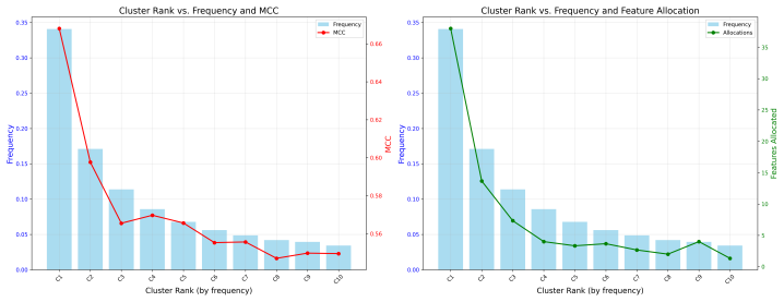
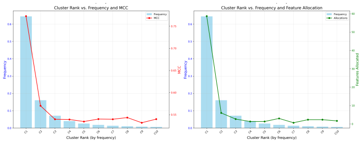
On the paper's own terms, the discovery is that feature consistency is not an unsolvable pathology but an attainable, measurable property, and that the path to it runs through architectural choices that enforce exact sparsity and zero reconstruction error. Theory adapted from sparse dictionary learning says a dictionary satisfying the spark condition, meaning no two distinct $k$-sparse codes produce the same output, is identifiable up to permutation and scaling once the data covers a certain witness set. The paper proves that a round-trip property, encoder(decoder($f$)) $=$ $f$ for every $k$-sparse $f$, implies the spark condition, and argues that TopK SAEs' training objective promotes exactly that. In synthetic matched settings TopK SAEs reach PW-MCC around 0.97; on LLM activations they reach around 0.80, with frequent features more consistent than rare ones, and high dictionary-vector similarity between matched features correlates with semantic similarity of their generated explanations.
Load-bearing premise
The consistency guarantee for TopK SAEs rests on assuming the training data contains, for every possible k-sparse code, an activation that the encoder maps to that code; on finite real datasets this exact reachability cannot hold, so the real-world experiments are an analogy to the theorem rather than an instance of it.
Editorial extensions
If this is right
- If PW-MCC is adopted as a standard evaluation number, SAE papers can be compared on reproducibility alongside reconstruction loss, and hyperparameters such as the TopK sparsity $k$ can be chosen where consistency peaks.
- Routine reporting of PW-MCC contextualized by feature frequency would turn feature interpretation from a one-off per-run activity into reusable annotations: stably matched features can be labeled once and carried across runs.
- Consistency-based evaluation would surface a frequency-dependent quality spectrum, with frequent features highly reproducible and rare-tail features less so, guiding where interpretability effort is best spent.
- Building interpretability claims such as circuits, steering, and unlearning on consistent dictionaries would make those claims robust to random initialization, addressing a documented failure mode where overlap between runs can be as low as 30 percent for standard SAEs.
Reading between the lines
- A natural but untested corollary is that consistency can also serve as a selection signal for data quality: if the same TopK recipe yields high PW-MCC on one layer or corpus and low on another, the lower value may indicate that the activation distribution lacks the coverage the identifiability theorem needs, not merely that training failed.
- The frequency-consistency spectrum suggests a division of labor for future SAE designs: reserve the dictionary's capacity for the frequent, stable core and treat the long tail as explicitly approximate, rather than expecting one architecture to be uniformly consistent.
- An obvious extension is to turn PW-MCC into a training objective or regularizer: because it is evaluated on a matched-pair basis, one could test whether adding a consistency-promoting penalty between concurrent runs raises PW-MCC, something the paper motivates but does not implement.
- Because the theory's reachability assumption is untestable on real data, the LLM results should be read as empirical evidence for an analogy rather than as a theorem instantiated.
Editorial analysis
A structured set of objections, weighed in public.
Referee Report
Summary. The paper argues that mechanistic interpretability (MI) should prioritize feature consistency in sparse autoencoders (SAEs), operationalized as the reliable convergence to equivalent feature sets across independent training runs. The authors propose the Pairwise Dictionary Mean Correlation Coefficient (PW-MCC) as a practical metric, provide a theoretical argument connecting SAE training to dictionary learning identifiability, present synthetic experiments showing PW-MCC tracks ground-truth recovery (GT-MCC), and report real-world experiments on Pythia-160M and Gemma-2-2B activations in which TopK SAEs achieve PW-MCC of about 0.80 and feature-level similarity correlates with semantic explanation similarity. The paper concludes with a call for the community to routinely report consistency metrics.
Significance. If the empirical findings hold, the paper offers a constructive resolution to a well-documented problem: learned SAE features are often unstable across runs, undermining reproducibility and cumulative progress. The release of code, the multi-seed protocol, and the comparison across seven architectures on two LLMs are strengths, as is the synthetic validation of PW-MCC against a known ground truth in a matched-capacity setting. The central position is plausible and potentially influential. However, the theoretical guarantee is conditional on idealized reachability and zero-error conditions that are not met in the real-world experiments, and the validity of PW-MCC as a proxy for ground-truth recovery is demonstrated only in a linear synthetic regime. The paper's practical force thus depends on additional empirical support that it does not yet provide.
major comments (3)
- [Section 4.1 and Appendix C, Corollary 1] The theoretical guarantee rests on conditions that are not satisfied in the experiments that the theory is invoked to support. Corollary 1 requires zero reconstruction error on the training set and reachability of every k-sparse code f, i.e., for all f in Sigma_k there exists x in X with E(x)=f. Appendix C.5 concedes that exact reachability cannot be verified on finite datasets, and the real-world SAE training (Section 5.2) does not achieve zero reconstruction error. Consequently, the claim that the theoretical analysis 'explains why TopK SAEs can achieve consistent features' (Section 4.1) is an analogy rather than a proof. Please either empirically check the conditions to the extent possible and report how far they are from being satisfied, or explicitly frame the theorem as an idealized sufficient condition and state that the real-data results are only suggestive.
- [Section 5.1 and Section 4.2] The statement that 'PW-MCC acts as a justifiable proxy for ground-truth alignment in unsupervised settings' is supported only by synthetic experiments with a linear generative model, exact k-sparse codes, and a matched-capacity regime (Section 4.2). Real LLM activations are not produced by such a generator, and the SAE operates in a globally compressive regime where d_SAE is far smaller than the number of latent concepts. The paper does not demonstrate that PW-MCC tracks GT-MCC in any setting resembling the LLM experiments. The semantic validation in Table 2 is partly circular: the same LLM (gpt-4.1) both generates and evaluates the explanations, and features with high dictionary-vector cosine similarity will have similar top-activating contexts mechanically, so high GPT scores are expected even if the learned features do not correspond to meaningful latent factors. Please add an external validation, e.g., a different judge LLM or human evaluation, or a synthetic benchmark with a more realistic generative process and known ground truth.
- [Section 5.2 and Appendix F.1] The headline PW-MCC values are the maximum over a hyperparameter sweep that was designed to maximize PW-MCC: 'For each SAE, we performed a hyperparameter sweep, selecting the configuration that yielded the highest final PW-MCC across three independent training runs.' Thus the reported 0.80 for TopK SAEs is an upper extreme, not a typical or average outcome, and the claim that 'high consistency is achievable' is inflated by selection. This matters because the paper's position is to prioritize consistency as an evaluation metric; showing that consistency can be optimized by searching hyperparameters is weaker than demonstrating that a standard configuration reliably yields high consistency. Please report the distribution of PW-MCC across the sweep (e.g., median and range) and state explicitly that the reported values were selected to maximize the metric.
minor comments (4)
- [Section 4.1] The sentence 'The training objective simultaneously encourages ... (2) Zero reconstruction error by minimizing ||X-AF||_F' is imprecise: minimizing an objective does not guarantee zero error unless the data lies in the span of the learned dictionary. Rephrase as 'aims to achieve zero reconstruction error.'
- [Table 2] The caption states that GPT-score is averaged over 20 pairs, but the number of feature pairs per similarity range is 34, 311, 975, 1,423, and 13,640. Please clarify how the 20-pair average is computed and whether the reported scores are based on a random subsample.
- [Appendix C.1] In the definition of the TopK encoder, the tie-breaking rule is specified as 'lexicographically' but the encoder selects the k largest magnitude inner products. It would be clearer to state that ties are broken deterministically by feature index.
- [Figure 4] The figure caption describes 'Token frequency in 1M tokens from Pile' but does not state which model's tokenizer or dataset split was used. Please add this detail for reproducibility.
Circularity Check
No significant circularity: PW-MCC validation uses external synthetic ground truth; the single self-citation is not load-bearing.
full rationale
PW-MCC is defined independently of fitted hyperparameters and ground-truth dictionaries in Section 3, so the consistency metric is not constructed to force the claimed outcome. The synthetic validation in Section 4.2 compares PW-MCC to GT-MCC against a known generative dictionary; this is an external empirical check, not a definitional identity. The theoretical argument in Section 4.1 and Appendix C is a conditional derivation adapted from the external identifiability result of Hillar and Sommer [22]; Appendix C proves that the round-trip property implies the spark condition, and Corollary 1 states that zero reconstruction error plus reachability imply the round-trip property. These are stated assumptions, not the conclusion. Appendix C.5 explicitly concedes that exact reachability cannot be verified on finite real data, so the real-world extension is an analogy and a limitation rather than a concealed circular step. The only self-citation is reference [37], used as an example of a downstream application in Section 3; it is not load-bearing for the consistency claim or the uniqueness theorem. The reported PW-MCC values in Section 5.2 are presented as achievable under a hyperparameter sweep selecting the configuration with the highest final PW-MCC, not as out-of-sample predictions. The semantic validation in Table 2 has a methodological confound because the same LLM generates and rates explanations based on the features being compared, but the paper does not use this as a formal derivation; it is a supporting correlation. Overall, no step in the paper's derivation chain reduces by construction to its own inputs, so the circularity burden is low.
Assumptions & free parameters
free parameters (4)
- TopK sparsity k (target L0) for real-data SAEs =
k=20 (Pythia-160M), k=80 (Gemma-2-2B)
- Sparsity penalty lambda for L1-based SAEs (Standard, Gated, P-Anneal) =
lambda=0.06 for Standard and Gated on Pythia-160M; lambda=0.03/0.04 for Standard/Gated on Gemma-2-2B; P-Anneal initial…
- Synthetic capacity allocation exponent beta =
beta approximately 1.25 to 1.46 depending on Zipf alpha
- Ground-truth sparsity s and dictionary dimensions in synthetic experiments =
s=8 for Zipf experiments, s=3 for matched regime (m=8, dgt=16)
assumptions (5)
- standard math A dictionary A is k-injective if and only if spark(A) > 2k
- standard math There exists a witness set of n = k * C(dsae,k)^2 k-sparse vectors such that any two spark-satisfying dictionaries factorizing X coincide up to permutation and scaling (Hillar-Sommer Theorem 1)
- ad hoc to paper The TopK encoder satisfies the round-trip property E(Af)=f on the training data, requiring zero reconstruction error and reachability of every k-sparse code
- domain assumption Natural language activation features follow a Zipfian distribution, motivating the model organism
- domain assumption Ground-truth dictionaries in synthetic experiments are i.i.d. Gaussian with unit-norm columns
Cite this review
Pith. "Pith review of Position: Mechanistic Interpretability Should Prioritize Feature Consistency in SAEs." pith.science (2026). https://pith.science/paper/5IEZ3NVZ
@misc{pith2026250520254,
  author       = {Pith},
  title        = {Pith review of: Position: Mechanistic Interpretability Should Prioritize Feature Consistency in SAEs},
  year         = {2026},
  howpublished = {\url{https://pith.science/paper/5IEZ3NVZ}},
  note         = {Machine review of arXiv:2505.20254}
}
read the original abstract
Sparse Autoencoders (SAEs) are a prominent tool in mechanistic interpretability (MI) for decomposing neural network activations into interpretable features. However, the aspiration to identify a canonical set of features is challenged by the observed inconsistency of learned SAE features across different training runs, undermining the reliability and efficiency of MI research. This position paper argues that mechanistic interpretability should prioritize feature consistency in SAEs -- the reliable convergence to equivalent feature sets across independent runs. We propose using the Pairwise Dictionary Mean Correlation Coefficient (PW-MCC) as a practical metric to operationalize consistency and demonstrate that high levels are achievable (0.80 for TopK SAEs on LLM activations) with appropriate architectural choices. Our contributions include detailing the benefits of prioritizing consistency; providing theoretical grounding and synthetic validation using a model organism, which verifies PW-MCC as a reliable proxy for ground-truth recovery; and extending these findings to real-world LLM data, where high feature consistency strongly correlates with the semantic similarity of learned feature explanations. We call for a community-wide shift towards systematically measuring feature consistency to foster robust cumulative progress in MI.
Figures


Figures from the paper (31 more)






Reference graph
Works this paper leans on
-
[1]
Samir Abdaljalil, Filippo Pallucchini, Andrea Seveso, Hasan Kurban, Fabio Mercorio, and Erchin Serpedin. Safe: A sparse autoencoder-based framework for robust query enrichment and hallucination mitigation in llms.arXiv preprint arXiv:2503.03032, 2025
arXiv 2025
-
[2]
Emmanuel Ameisen, Jack Lindsey, Adam Pearce, Wes Gurnee, Nicholas L. Turner, Brian Chen, Craig Citro, David Abrahams, Shan Carter, Basil Hosmer, Jonathan Marcus, Michael Sklar, Adly Templeton, Trenton Bricken, Callum McDougall, Hoagy Cunningham, Thomas Henighan, Adam Jermyn, Andy Jones, Andrew Persic, Zhenyi Qi, T. Ben Thompson, Sam Zimmerman, Kelley Rivo...
work page 2025
-
[3]
New algorithms for learning incoherent and overcomplete dictionaries
Sanjeev Arora, Rong Ge, and Ankur Moitra. New algorithms for learning incoherent and overcomplete dictionaries. InConference on Learning Theory, pages 779–806. PMLR, 2014
2014
-
[4]
Pythia: A suite for analyzing large language models across training and scaling
Stella Biderman, Hailey Schoelkopf, Quentin Anthony, Herbie Bradley, Kyle O’Brien, Eric Hallahan, Mohammad Aflah Khan, Shivanshu Purohit, USVSN Sai Prashanth, Edward Raff, et al. Pythia: A suite for analyzing large language models across training and scaling. In Proceedings of the 40th International Conference on Machine Learning, ICML’23, 2023. 10
work page 2023
-
[5]
Turner, Cem Anil, Carson Denison, Amanda Askell, et al
Trenton Bricken, Adly Templeton, Joshua Batson, Brian Chen, Adam Jermyn, Tom Conerly, Nicholas L. Turner, Cem Anil, Carson Denison, Amanda Askell, et al. Towards monoseman- ticity: Decomposing language models with dictionary learning.Transformer Circuits Thread, 2023
work page 2023
-
[6]
Towards monosemanticity: Decomposing language models with dictionary learning
Trenton Bricken, Adly Templeton, Joshua Batson, Brian Chen, Adam Jermyn, Tom Conerly, Nicholas L Turner, Cem Anil, Carson Denison, Amanda Askell, Robert Lasenby, Yifan Wu, Shauna Kravec, Nicholas Schiefer, Tim Maxwell, Nicholas Joseph, Alex Tamkin, Karina Nguyen, Brayden McLean, Josiah E Burke, Tristan Hume, Shan Carter, Tom Henighan, and Chris Olah. Towa...
work page 2023
-
[7]
Batchtopk sparse autoencoders.arXiv preprint arXiv:2412.06410, 2024
Bart Bussmann, Patrick Leask, and Neel Nanda. Batchtopk sparse autoencoders.arXiv preprint arXiv:2412.06410, 2024
arXiv 2024
-
[8]
Bart Bussmann, Noa Nabeshima, Adam Karvonen, and Neel Nanda. Learning multi-level features with matryoshka sparse autoencoders.arXiv preprint arXiv:2503.17547, 2025
arXiv 2025
Show all 56 references
-
[9]
Improving steering vectors by targeting sparse autoencoder features.arXiv preprint arXiv:2411.02193, 2024
Sviatoslav Chalnev, Matthew Siu, and Arthur Conmy. Improving steering vectors by targeting sparse autoencoder features.arXiv preprint arXiv:2411.02193, 2024
2024 arXiv
-
[10]
A is for absorption: Studying feature splitting and absorption in sparse autoencoders.arXiv preprint arXiv:2409.14507, 2024
David Chanin, James Wilken-Smith, Tomáš Dulka, Hardik Bhatnagar, and Joseph Bloom. A is for absorption: Studying feature splitting and absorption in sparse autoencoders.arXiv preprint arXiv:2409.14507, 2024
2024
-
[11]
Sparse autoen- coders find highly interpretable features in language models.arXiv preprint arXiv:2309.08600, 2023
Hoagy Cunningham, Aidan Ewart, Logan Riggs, Robert Huben, and Lee Sharkey. Sparse autoen- coders find highly interpretable features in language models.arXiv preprint arXiv:2309.08600, 2023
2023 arXiv
-
[12]
Optimally sparse representation in general (nonorthogonal) dictionaries via l1 minimization.Proceedings of the National Academy of Sciences, 100(5):2197– 2202, 2003
David L Donoho and Michael Elad. Optimally sparse representation in general (nonorthogonal) dictionaries via l1 minimization.Proceedings of the National Academy of Sciences, 100(5):2197– 2202, 2003
2003
-
[13]
Toy models of superposition.arXiv preprint arXiv:2209.10652, 2022
Nelson Elhage, Tristan Hume, Catherine Olsson, Nicholas Schiefer, Tom Henighan, Shauna Kravec, Zac Hatfield-Dodds, Robert Lasenby, Dawn Drain, Carol Chen, et al. Toy models of superposition.arXiv preprint arXiv:2209.10652, 2022
2022 arXiv
-
[14]
A mathematical framework for transformer circuits.Transformer Circuits Thread, 1(1):12, 2021
Nelson Elhage, Neel Nanda, Catherine Olsson, Tom Henighan, Nicholas Joseph, Ben Mann, Amanda Askell, Yuntao Bai, Anna Chen, Tom Conerly, et al. A mathematical framework for transformer circuits.Transformer Circuits Thread, 1(1):12, 2021
2021
-
[15]
Archetypal sae: Adaptive and stable dictionary learning for concept extraction in large vision models.arXiv preprint arXiv:2502.12892, 2025
Thomas Fel, Ekdeep Singh Lubana, Jacob S Prince, Matthew Kowal, Victor Boutin, Isabel Papadimitriou, Binxu Wang, Martin Wattenberg, Demba Ba, and Talia Konkle. Archetypal sae: Adaptive and stable dictionary learning for concept extraction in large vision models.arXiv preprint ...
2025 arXiv
-
[16]
Scientific inference with interpretable machine learning: Analyzing models to learn about real-world phenomena.Minds and Machines, 34(3):32, 2024
Timo Freiesleben, Gunnar König, Christoph Molnar, and Alvaro Tejero-Cantero. Scientific inference with interpretable machine learning: Analyzing models to learn about real-world phenomena.Minds and Machines, 34(3):32, 2024
2024
-
[17]
The pile: An 800gb dataset of diverse text for language modeling.arXiv preprint arXiv:2101.00027, 2020
Leo Gao, Stella Biderman, Sid Black, Laurence Golding, Travis Hoppe, Charles Foster, Jason Phang, Horace He, Anish Thite, Noa Nabeshima, et al. The pile: An 800gb dataset of diverse text for language modeling.arXiv preprint arXiv:2101.00027, 2020
2020 arXiv
-
[18]
Scaling and evaluating sparse autoencoders.arXiv preprint arXiv:2406.04093, 2024
Leo Gao, Tom Dupré la Tour, Henk Tillman, Gabriel Goh, Rajan Troll, Alec Radford, Ilya Sutskever, Jan Leike, and Jeffrey Wu. Scaling and evaluating sparse autoencoders.arXiv preprint arXiv:2406.04093, 2024
2024 arXiv
-
[19]
Scaling and evaluating sparse autoencoders
Leo Gao, Tom Dupre la Tour, Henk Tillman, Gabriel Goh, Rajan Troll, Alec Radford, Ilya Sutskever, Jan Leike, and Jeffrey Wu. Scaling and evaluating sparse autoencoders. InThe Thirteenth International Conference on Learning Representations, 2025. 11
2025
-
[20]
Causal abstraction: A theoretical foundation for mechanistic interpretability.arXiv preprint arXiv:2301.04709, 2023
Atticus Geiger, Duligur Ibeling, Amir Zur, Maheep Chaudhary, Sonakshi Chauhan, Jing Huang, Aryaman Arora, Zhengxuan Wu, Noah Goodman, Christopher Potts, et al. Causal abstraction: A theoretical foundation for mechanistic interpretability.arXiv preprint arXiv:2301.04709, 2023
2023 arXiv
-
[21]
Scar: Sparse conditioned autoencoders for concept detection and steering in llms.arXiv preprint arXiv:2411.07122, 2024
Ruben Härle, Felix Friedrich, Manuel Brack, Björn Deiseroth, Patrick Schramowski, and Kristian Kersting. Scar: Sparse conditioned autoencoders for concept detection and steering in llms.arXiv preprint arXiv:2411.07122, 2024
2024 arXiv
-
[22]
When can dictionary learning uniquely recover sparse data from subsamples?IEEE Transactions on Information Theory, 61(11):6290–6297, 2015
Christopher J Hillar and Friedrich T Sommer. When can dictionary learning uniquely recover sparse data from subsamples?IEEE Transactions on Information Theory, 61(11):6290–6297, 2015
2015
-
[23]
Projecting assumptions: The duality between sparse autoencoders and concept geometry.arXiv preprint arXiv:2503.01822, 2025
Sai Sumedh R Hindupur, Ekdeep Singh Lubana, Thomas Fel, and Demba Ba. Projecting assumptions: The duality between sparse autoencoders and concept geometry.arXiv preprint arXiv:2503.01822, 2025
2025
-
[24]
Independent component analysis: algorithms and applications
Aapo Hyvärinen and Erkki Oja. Independent component analysis: algorithms and applications. Neural networks, 13(4-5):411–430, 2000
2000
-
[25]
Identifiable steering via sparse autoencoding of multi-concept shifts.arXiv preprint arXiv:2502.12179, 2025
Shruti Joshi, Andrea Dittadi, Sébastien Lachapelle, and Dhanya Sridhar. Identifiable steering via sparse autoencoding of multi-concept shifts.arXiv preprint arXiv:2502.12179, 2025
2025
-
[26]
SAEBench: A Comprehensive Benchmark for Sparse Autoencoders.https://www.neuronpedia.org/sae-bench/info, 2024
Adam Karvonen, Can Rager, Jessica Lin, Curt Tigges, Jacob Bloom, Daniel Chanin, Yue- Ting Lau, Euan Farrell, Arthur Conmy, Callum McDougall, Kolawole Ayonrinde, Martin Wearden, Logan Marks, and Neel Nanda. SAEBench: A Comprehensive Benchmark for Sparse Autoencoders.https://www...
2024
-
[27]
Measuring progress in dictionary learning for language model interpretability with board game models.Advances in Neural Information Processing Systems, 37:83091–83118, 2024
Adam Karvonen, Benjamin Wright, Can Rager, Rico Angell, Jannik Brinkmann, Logan Smith, Claudio Mayrink Verdun, David Bau, and Samuel Marks. Measuring progress in dictionary learning for language model interpretability with board game models.Advances in Neural Information Proce...
2024
-
[28]
Sparse autoencoders do not find canonical units of analysis.arXiv preprint arXiv:2502.04878, 2025
Patrick Leask, Bart Bussmann, Michael Pearce, Joseph Bloom, Curt Tigges, Noura Al Moubayed, Lee Sharkey, and Neel Nanda. Sparse autoencoders do not find canonical units of analysis.arXiv preprint arXiv:2502.04878, 2025
2025 arXiv
-
[29]
Jack Lindsey, Wes Gurnee, Emmanuel Ameisen, Brian Chen, Adam Pearce, Nicholas L. Turner, Craig Citro, David Abrahams, Shan Carter, Basil Hosmer, Jonathan Marcus, Michael Sklar, Adly Templeton, Trenton Bricken, Callum McDougall, Hoagy Cunningham, Thomas Henighan, Adam Jermyn, A...
2025
-
[30]
The mythos of model interpretability: In machine learning, the concept of interpretability is both important and slippery.Queue, 16(3):31–57, 2018
Zachary C Lipton. The mythos of model interpretability: In machine learning, the concept of interpretability is both important and slippery.Queue, 16(3):31–57, 2018
2018
-
[31]
Is this the subspace you are looking for? an interpretability illusion for subspace activation patching.arXiv preprint arXiv:2311.17030, 2023
Aleksandar Makelov, Georg Lange, and Neel Nanda. Is this the subspace you are looking for? an interpretability illusion for subspace activation patching.arXiv preprint arXiv:2311.17030, 2023
2023 arXiv
-
[32]
Enhancing neural network interpretability with feature-aligned sparse autoencoders.arXiv preprint arXiv:2411.01220, 2024
Luke Marks, Alasdair Paren, David Krueger, and Fazl Barez. Enhancing neural network interpretability with feature-aligned sparse autoencoders.arXiv preprint arXiv:2411.01220, 2024
2024 arXiv
-
[33]
Dictionary learning
Samuel Marks, Adam Karvonen, and Aaron Mueller. Dictionary learning. https://github. com/saprmarks/dictionary_learning, 2024
2024
-
[34]
Sparse feature circuits: Discovering and editing interpretable causal graphs in language models
Samuel Marks, Can Rager, Eric J Michaud, Yonatan Belinkov, David Bau, and Aaron Mueller. Sparse feature circuits: Discovering and editing interpretable causal graphs in language models. arXiv preprint arXiv:2403.19647, 2024. 12
2024 arXiv
-
[35]
Sparse feature circuits: Discovering and editing interpretable causal graphs in language models
Samuel Marks, Can Rager, Eric J Michaud, Yonatan Belinkov, David Bau, and Aaron Mueller. Sparse feature circuits: Discovering and editing interpretable causal graphs in language models. InThe Thirteenth International Conference on Learning Representations, 2025
2025
-
[36]
Everything, everywhere, all at once: Is mechanistic interpretability identifiable?arXiv preprint arXiv:2502.20914, 2025
Maxime Méloux, Silviu Maniu, François Portet, and Maxime Peyrard. Everything, everywhere, all at once: Is mechanistic interpretability identifiable?arXiv preprint arXiv:2502.20914, 2025
2025 arXiv
-
[37]
Saes can improve unlearn- ing: Dynamic sparse autoencoder guardrails for precision unlearning in llms.arXiv preprint arXiv:2504.08192, 2025
Aashiq Muhamed, Jacopo Bonato, Mona Diab, and Virginia Smith. Saes can improve unlearn- ing: Dynamic sparse autoencoder guardrails for precision unlearning in llms.arXiv preprint arXiv:2504.08192, 2025
2025 arXiv
-
[38]
Steering language model refusal with sparse autoencoders.arXiv preprint arXiv:2411.11296, 2024
Kyle O’Brien, David Majercak, Xavier Fernandes, Richard Edgar, Jingya Chen, Harsha Nori, Dean Carignan, Eric Horvitz, and Forough Poursabzi-Sangde. Steering language model refusal with sparse autoencoders.arXiv preprint arXiv:2411.11296, 2024
2024 arXiv
-
[39]
Mechanistic interpretability, variables, and the importance of interpretable bases
Chris Olah. Mechanistic interpretability, variables, and the importance of interpretable bases. Transformer Circuits Thread, 2(4), 2022
2022
-
[40]
Zoom in: An introduction to circuits.Distill, 5(3):e00024–001, 2020
Chris Olah, Nick Cammarata, Ludwig Schubert, Gabriel Goh, Michael Petrov, and Shan Carter. Zoom in: An introduction to circuits.Distill, 5(3):e00024–001, 2020
2020
-
[41]
The building blocks of interpretability.Distill, 3(3):e10, 2018
Chris Olah, Arvind Satyanarayan, Ian Johnson, Shan Carter, Ludwig Schubert, Katherine Ye, and Alexander Mordvintsev. The building blocks of interpretability.Distill, 3(3):e10, 2018
2018
-
[42]
Compute optimal inference and provable amortisation gap in sparse autoencoders.arXiv preprint arXiv:2411.13117, 2024
Charles O’Neill, Alim Gumran, and David Klindt. Compute optimal inference and provable amortisation gap in sparse autoencoders.arXiv preprint arXiv:2411.13117, 2024
2024 arXiv
-
[43]
Sparse autoencoders learn monosemantic features in vision-language models.arXiv preprint arXiv:2504.02821, 2025
Mateusz Pach, Shyamgopal Karthik, Quentin Bouniot, Serge Belongie, and Zeynep Akata. Sparse autoencoders learn monosemantic features in vision-language models.arXiv preprint arXiv:2504.02821, 2025
2025
-
[44]
Sparse autoencoders trained on the same data learn different features.arXiv preprint arXiv:2501.16615, 2025
Gonçalo Paulo and Nora Belrose. Sparse autoencoders trained on the same data learn different features.arXiv preprint arXiv:2501.16615, 2025
2025 arXiv
-
[45]
Automatically interpreting millions of features in large language models.arXiv preprint arXiv:2410.13928, 2024
Gonçalo Paulo, Alex Mallen, Caden Juang, and Nora Belrose. Automatically interpreting millions of features in large language models.arXiv preprint arXiv:2410.13928, 2024
2024 arXiv
-
[46]
Improving dictionary learning with gated sparse autoencoders.arXiv preprint arXiv:2404.16014, 2024
Senthooran Rajamanoharan, Arthur Conmy, Lewis Smith, Tom Lieberum, Vikrant Varma, János Kramár, Rohin Shah, and Neel Nanda. Improving dictionary learning with gated sparse autoencoders.arXiv preprint arXiv:2404.16014, 2024
2024 arXiv
-
[47]
Jumping ahead: Improving reconstruction fidelity with jumprelu sparse autoencoders.arXiv preprint arXiv:2407.14435, 2024
Senthooran Rajamanoharan, Tom Lieberum, Nicolas Sonnerat, Arthur Conmy, Vikrant Varma, János Kramár, and Neel Nanda. Jumping ahead: Improving reconstruction fidelity with jumprelu sparse autoencoders.arXiv preprint arXiv:2407.14435, 2024
2024 arXiv
-
[48]
Global identifiability of overcomplete dictionary learning via l1 and volume minimization
Yuchen Sun and Kejun Huang. Global identifiability of overcomplete dictionary learning via l1 and volume minimization. InThe Twelfth International Conference on Learning Representations (ICLR), 2024
2024
-
[49]
Gemma: Open models based on gemini research and technology.arXiv preprint arXiv:2403.08295, 2024
Gemma Team, Thomas Mesnard, Cassidy Hardin, Robert Dadashi, Surya Bhupatiraju, Shreya Pathak, Laurent Sifre, Morgane Rivière, Mihir Sanjay Kale, Juliette Love, et al. Gemma: Open models based on gemini research and technology.arXiv preprint arXiv:2403.08295, 2024
2024 arXiv
-
[50]
Identifiability of overcomplete independent component analysis
Kexin Wang and Anna Seigal. Identifiability of overcomplete independent component analysis. arXiv preprint arXiv:2401.14709, 2024. 13 A Additional Related Work A.1 Sparse Autoencoders for Mechanistic Interpretability This section provides further context on the specific SAE ar...
2024 arXiv
-
[53]
Only the most frequent clusters show consistent reproducibility, indicating severe capacity limitations where the dictionary should prioritize only the dominant clusters
With small dictionary sizes (80-160 features), we observe only a weak relationship between activation frequency and feature reproducibility. Only the most frequent clusters show consistent reproducibility, indicating severe capacity limitations where the dictionary should prio...
-
[54]
As dictionary size increases to 1000 features, the relationship between activation frequency and reproducibility becomes more pronounced. A wider range of moderately frequent features begins to show improved reproducibility, as the increased capacity allows the model to repres...
-
[55]
The substantial increase in capacity 28 Figure 31:Two-phase model with dictionary size
At dictionary size 10000, we observe a positive relationship between activation frequency and reproducibility across a wide frequency range. The substantial increase in capacity 28 Figure 31:Two-phase model with dictionary size
-
[80]
Figure 30:Two-phase model with dictionary size
Feature reproducibility shows a weak positive relationship with activation frequency. Figure 30:Two-phase model with dictionary size
-
[160]
Figures 29 through 32 demonstrate how dictionary size affects feature reproducibility across the activation frequency spectrum
The relationship between activation frequency and feature reproducibility remains weak but becomes slightly more pronounced compared to dictionary size 80. Figures 29 through 32 demonstrate how dictionary size affects feature reproducibility across the activation frequency spe...
-
[1000]
the same
Feature reproducibility shows a moderately strong positive correlation with activation frequency especially at higher activation frequencies. Increased model capacity creates sufficient local redundancy for high probability clusters. Figure 32:Two-phase model with dictionary s...
2025
Reviewed August 7, 2026 · model on record in the stance chip above.
Discussion (0). Sign in to comment.